Statistical Analysis for Decision Support Tool: Probability

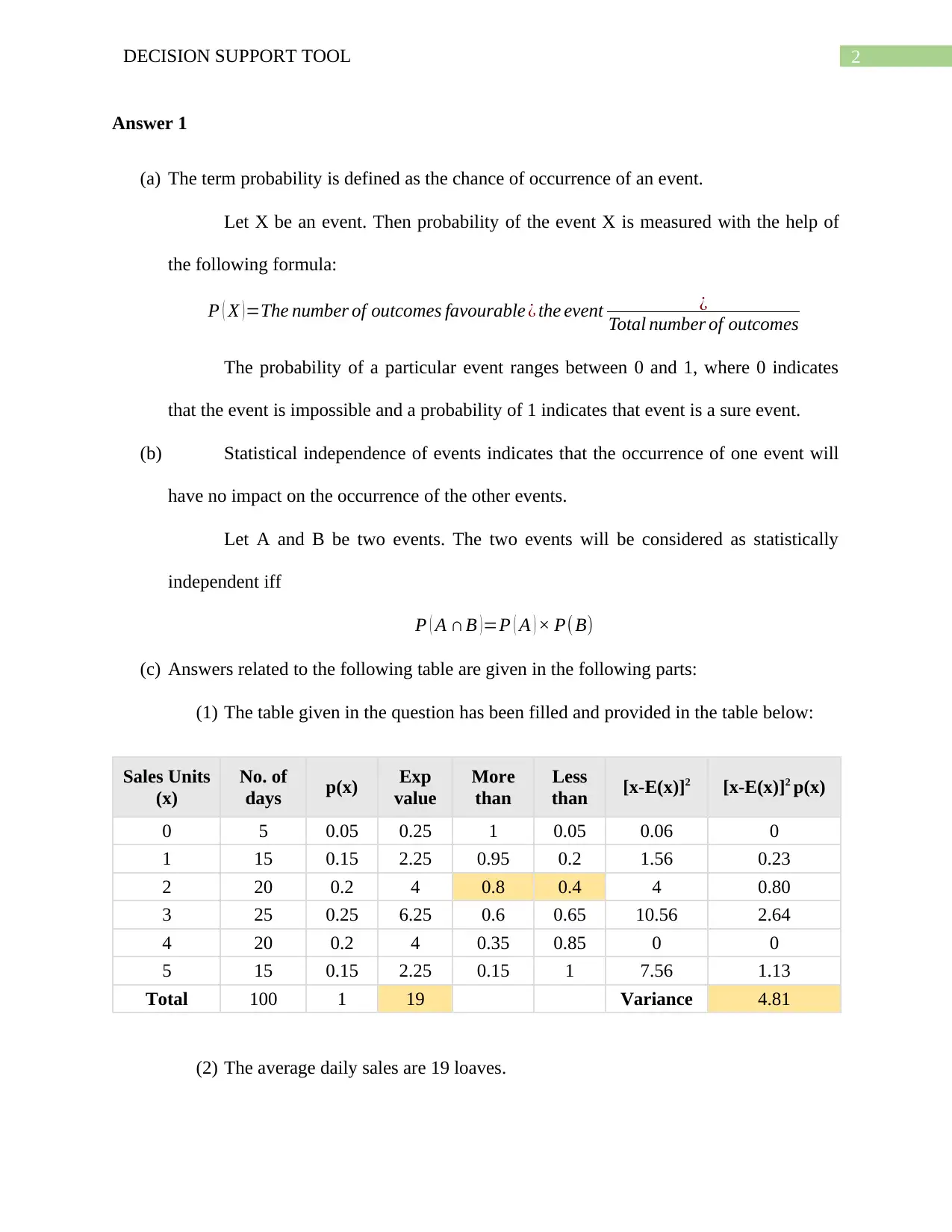
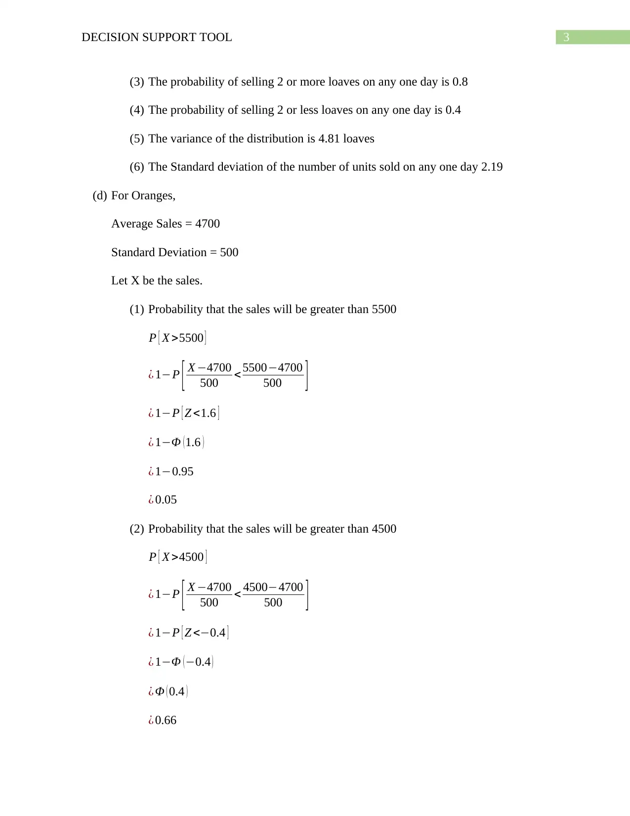
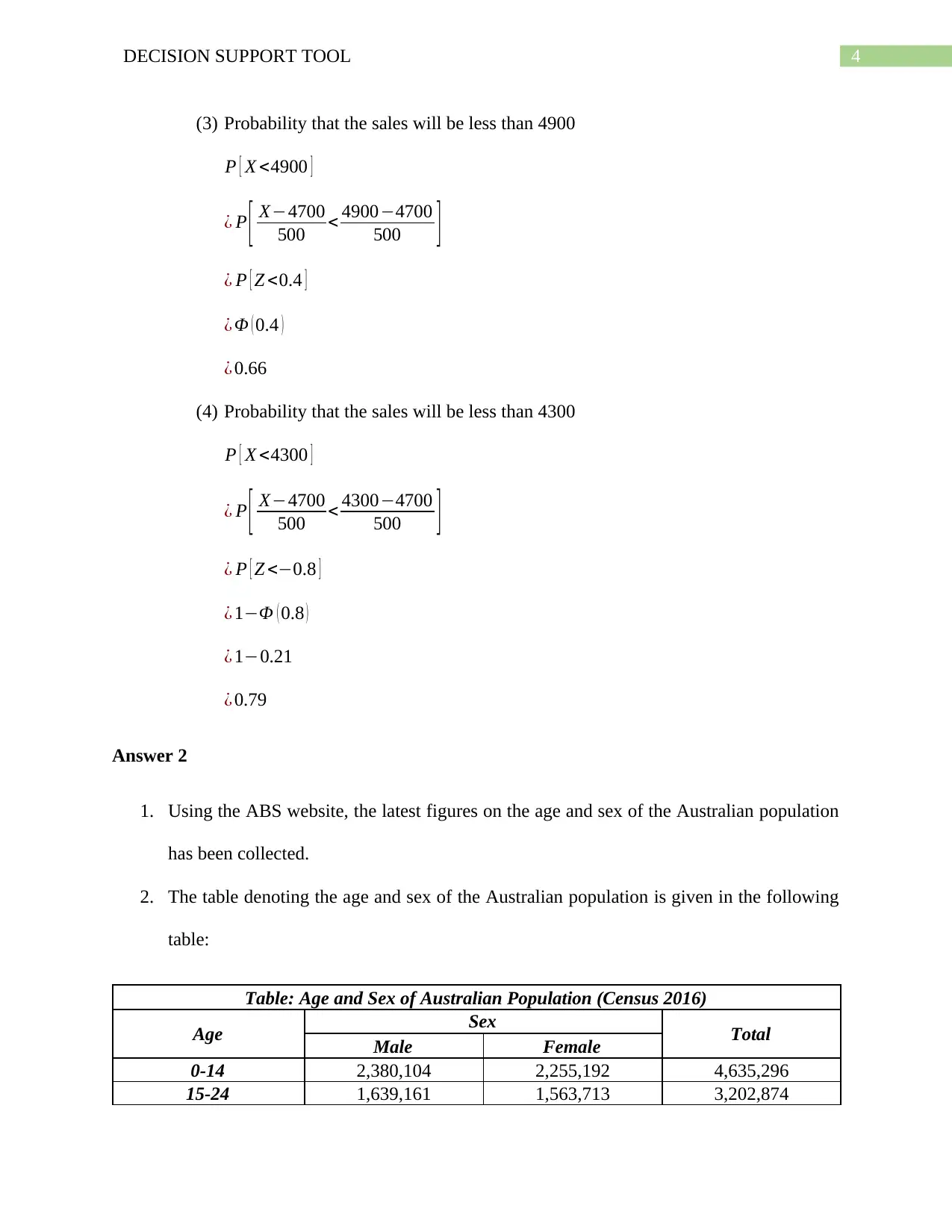
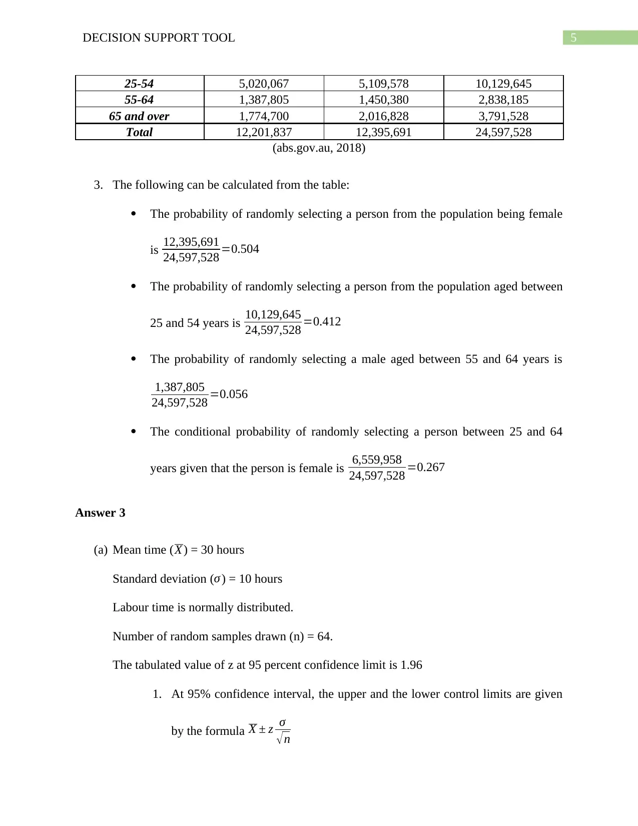
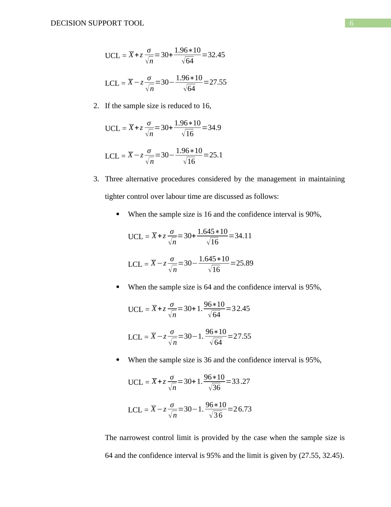
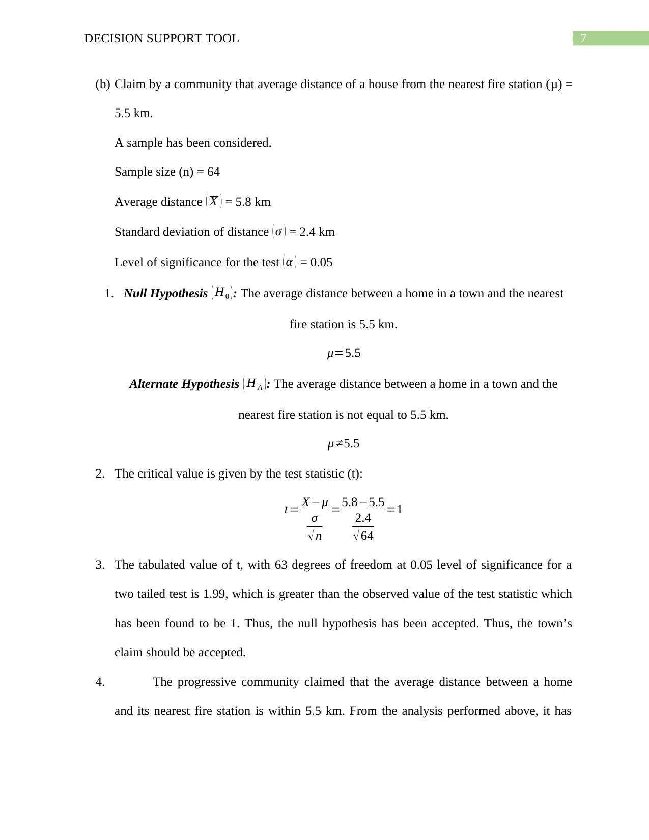
This assignment focuses on a decision support tool, delving into probability and statistical analysis. It covers fundamental concepts such as the definition of probability, statistical independence of events, and calculations involving probability distributions. The assignment includes a detailed analysis of sales data, calculating probabilities, variance, and standard deviation. Furthermore, it examines the age and sex distribution of the Australian population using data from the ABS website, computing various probabilities. The assignment also addresses statistical process control, determining upper and lower control limits for labor time, and hypothesis testing, evaluating a community's claim about the average distance to the nearest fire station. The solution provides comprehensive calculations, interpretations, and conclusions based on statistical principles. Desklib offers this and many more solved assignments and study tools for students.

Running Head: DECISION SUPPORT TOOL
Decision Support Tool
Name of the Student
Name of the University
Student ID

1DECISION SUPPORT TOOL
Table of Contents
Answer 1..........................................................................................................................................2
Answer 2..........................................................................................................................................4
Answer 3..........................................................................................................................................5
References........................................................................................................................................8

2DECISION SUPPORT TOOL
Answer 1
(a) The term probability is defined as the chance of occurrence of an event.
Let X be an event. Then probability of the event X is measured with the help of
the following formula:
P ( X ) =The number of outcomes favourable ¿ the event ¿
Total number of outcomes
The probability of a particular event ranges between 0 and 1, where 0 indicates
that the event is impossible and a probability of 1 indicates that event is a sure event.
(b) Statistical independence of events indicates that the occurrence of one event will
have no impact on the occurrence of the other events.
Let A and B be two events. The two events will be considered as statistically
independent iff
P ( A ∩B )=P ( A ) × P( B)
(c) Answers related to the following table are given in the following parts:
(1) The table given in the question has been filled and provided in the table below:
Sales Units
(x)
No. of
days p(x) Exp
value
More
than
Less
than [x-E(x)]2 [x-E(x)]2 p(x)
0 5 0.05 0.25 1 0.05 0.06 0
1 15 0.15 2.25 0.95 0.2 1.56 0.23
2 20 0.2 4 0.8 0.4 4 0.80
3 25 0.25 6.25 0.6 0.65 10.56 2.64
4 20 0.2 4 0.35 0.85 0 0
5 15 0.15 2.25 0.15 1 7.56 1.13
Total 100 1 19 Variance 4.81
(2) The average daily sales are 19 loaves.

3DECISION SUPPORT TOOL
(3) The probability of selling 2 or more loaves on any one day is 0.8
(4) The probability of selling 2 or less loaves on any one day is 0.4
(5) The variance of the distribution is 4.81 loaves
(6) The Standard deviation of the number of units sold on any one day 2.19
(d) For Oranges,
Average Sales = 4700
Standard Deviation = 500
Let X be the sales.
(1) Probability that the sales will be greater than 5500
P [ X >5500 ]
¿ 1−P [ X −4700
500 < 5500−4700
500 ]
¿ 1−P [ Z <1.6 ]
¿ 1−Φ (1.6 )
¿ 1−0.95
¿ 0.05
(2) Probability that the sales will be greater than 4500
P [ X >4500 ]
¿ 1−P [ X −4700
500 < 4500−4700
500 ]
¿ 1−P [ Z <−0.4 ]
¿ 1−Φ (−0.4 )
¿ Φ ( 0.4 )
¿ 0.66

4DECISION SUPPORT TOOL
(3) Probability that the sales will be less than 4900
P [ X <4900 ]
¿ P [ X−4700
500 < 4900−4700
500 ]
¿ P [ Z <0.4 ]
¿ Φ ( 0.4 )
¿ 0.66
(4) Probability that the sales will be less than 4300
P [ X <4300 ]
¿ P [ X−4700
500 < 4300−4700
500 ]
¿ P [ Z <−0.8 ]
¿ 1−Φ ( 0.8 )
¿ 1−0.21
¿ 0.79
Answer 2
1. Using the ABS website, the latest figures on the age and sex of the Australian population
has been collected.
2. The table denoting the age and sex of the Australian population is given in the following
table:
Table: Age and Sex of Australian Population (Census 2016)
Age Sex Total
Male Female
0-14 2,380,104 2,255,192 4,635,296
15-24 1,639,161 1,563,713 3,202,874

5DECISION SUPPORT TOOL
25-54 5,020,067 5,109,578 10,129,645
55-64 1,387,805 1,450,380 2,838,185
65 and over 1,774,700 2,016,828 3,791,528
Total 12,201,837 12,395,691 24,597,528
(abs.gov.au, 2018)
3. The following can be calculated from the table:
 The probability of randomly selecting a person from the population being female
is 12,395,691
24,597,528 =0.504
 The probability of randomly selecting a person from the population aged between
25 and 54 years is 10,129,645
24,597,528 =0.412
 The probability of randomly selecting a male aged between 55 and 64 years is
1,387,805
24,597,528 =0.056
 The conditional probability of randomly selecting a person between 25 and 64
years given that the person is female is 6,559,958
24,597,528 =0.267
Answer 3
(a) Mean time (X ) = 30 hours
Standard deviation (σ ) = 10 hours
Labour time is normally distributed.
Number of random samples drawn (n) = 64.
The tabulated value of z at 95 percent confidence limit is 1.96
1. At 95% confidence interval, the upper and the lower control limits are given
by the formula X ± z σ
√ n

6DECISION SUPPORT TOOL
UCL = X + z σ
√n =30+ 1.96∗10
√64 =32.45
LCL = X −z σ
√ n =30− 1.96∗10
√ 64 =27.55
2. If the sample size is reduced to 16,
UCL = X + z σ
√n =30+ 1.96∗10
√16 =34.9
LCL = X −z σ
√ n =30− 1.96∗10
√16 =25.1
3. Three alternative procedures considered by the management in maintaining
tighter control over labour time are discussed as follows:
 When the sample size is 16 and the confidence interval is 90%,
UCL = X + z σ
√n =30+ 1.645∗10
√16 =34.11
LCL = X −z σ
√ n =30− 1.645∗10
√16 =25.89
 When the sample size is 64 and the confidence interval is 95%,
UCL = X + z σ
√n =30+ 1. 96∗10
√64 =3 2.45
LCL = X −z σ
√ n =30−1. 96∗10
√ 64 =27.55
 When the sample size is 36 and the confidence interval is 95%,
UCL = X + z σ
√n =30+ 1. 96∗10
√36 =33 .27
LCL = X −z σ
√ n =30−1. 96∗10
√ 3 6 =2 6.73
The narrowest control limit is provided by the case when the sample size is
64 and the confidence interval is 95% and the limit is given by (27.55, 32.45).

7DECISION SUPPORT TOOL
(b) Claim by a community that average distance of a house from the nearest fire station (μ) =
5.5 km.
A sample has been considered.
Sample size (n) = 64
Average distance ( X ) = 5.8 km
Standard deviation of distance ( σ ) = 2.4 km
Level of significance for the test ( α ) = 0.05
1. Null Hypothesis ( H0 ): The average distance between a home in a town and the nearest
fire station is 5.5 km.
μ=5.5
Alternate Hypothesis ( H A ): The average distance between a home in a town and the
nearest fire station is not equal to 5.5 km.
μ ≠5.5
2. The critical value is given by the test statistic (t):
t= X−μ
σ
√ n
=5.8−5.5
2.4
√ 64
=1
3. The tabulated value of t, with 63 degrees of freedom at 0.05 level of significance for a
two tailed test is 1.99, which is greater than the observed value of the test statistic which
has been found to be 1. Thus, the null hypothesis has been accepted. Thus, the town’s
claim should be accepted.
4. The progressive community claimed that the average distance between a home
and its nearest fire station is within 5.5 km. From the analysis performed above, it has

8DECISION SUPPORT TOOL
been found out that the claim made by the community has been accepted. This indicates
that enough evidences have been found to confirm the claim made by the community.
5.

9DECISION SUPPORT TOOL
References
Abs.gov.au. (2018). 3101.0 - Australian Demographic Statistics, Dec 2017. [online] Available
at: http://www.abs.gov.au/AUSSTATS/abs@.nsf/DetailsPage/3101.0Dec 2017?OpenDocument
[Accessed 7 Aug. 2018].