Decision Support Systems: Project on Predictive Modeling and Analysis

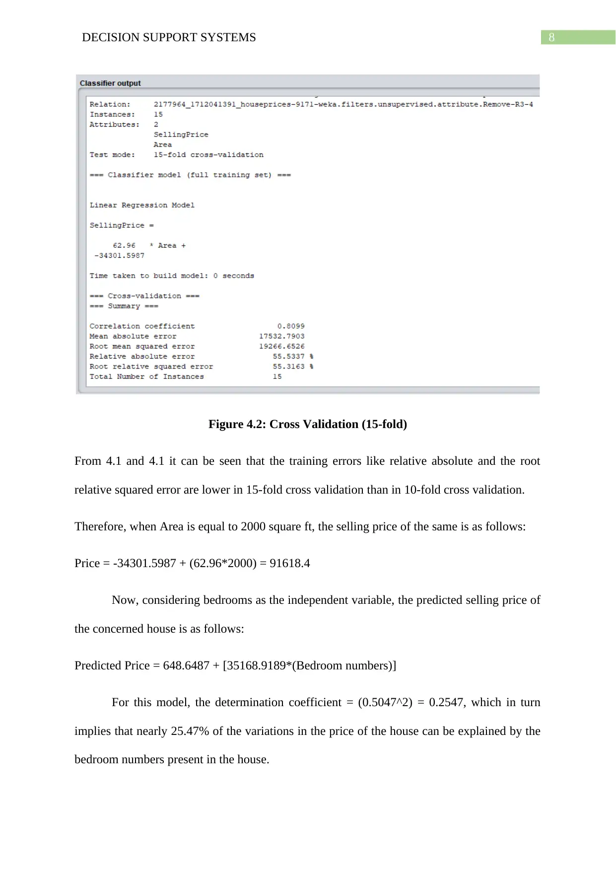
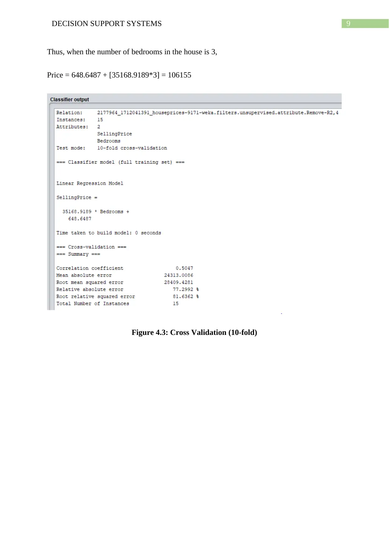
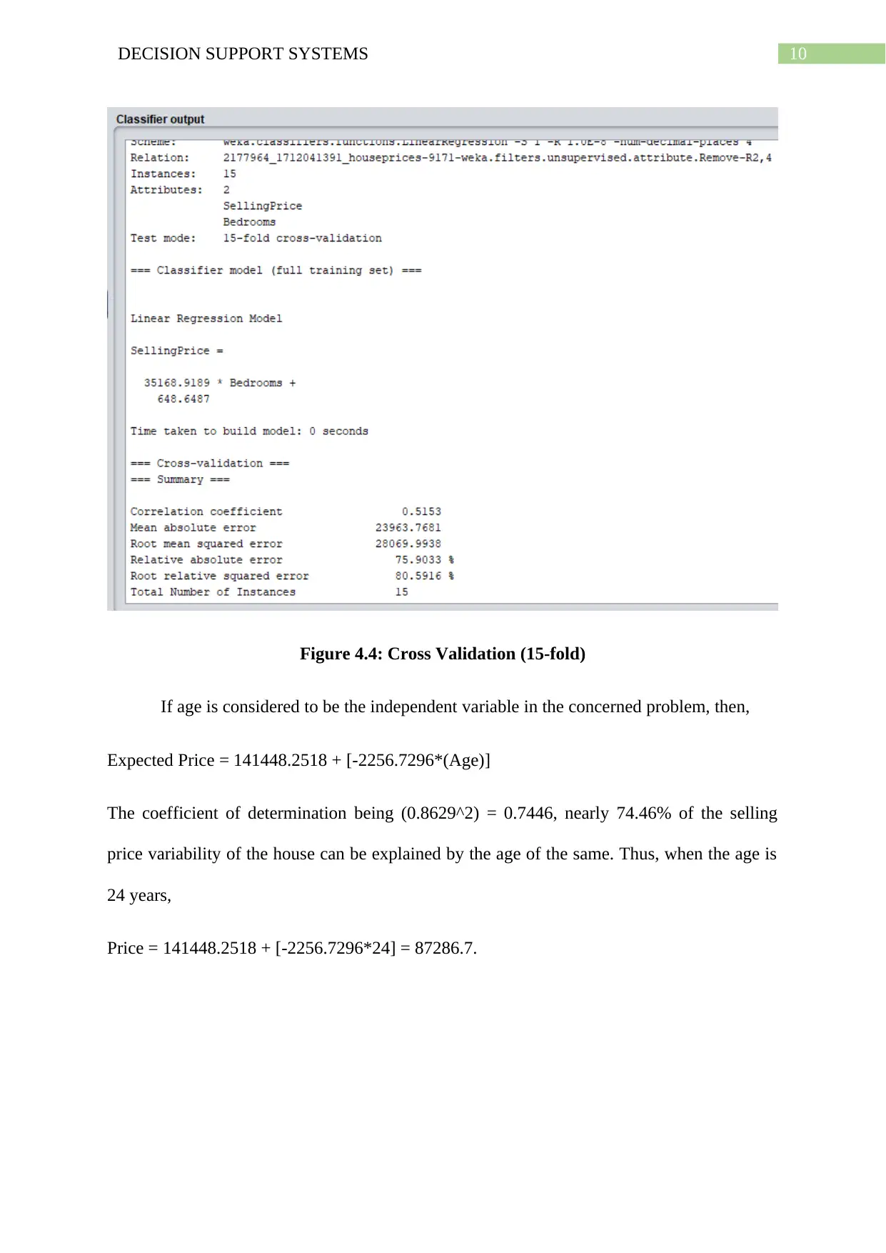
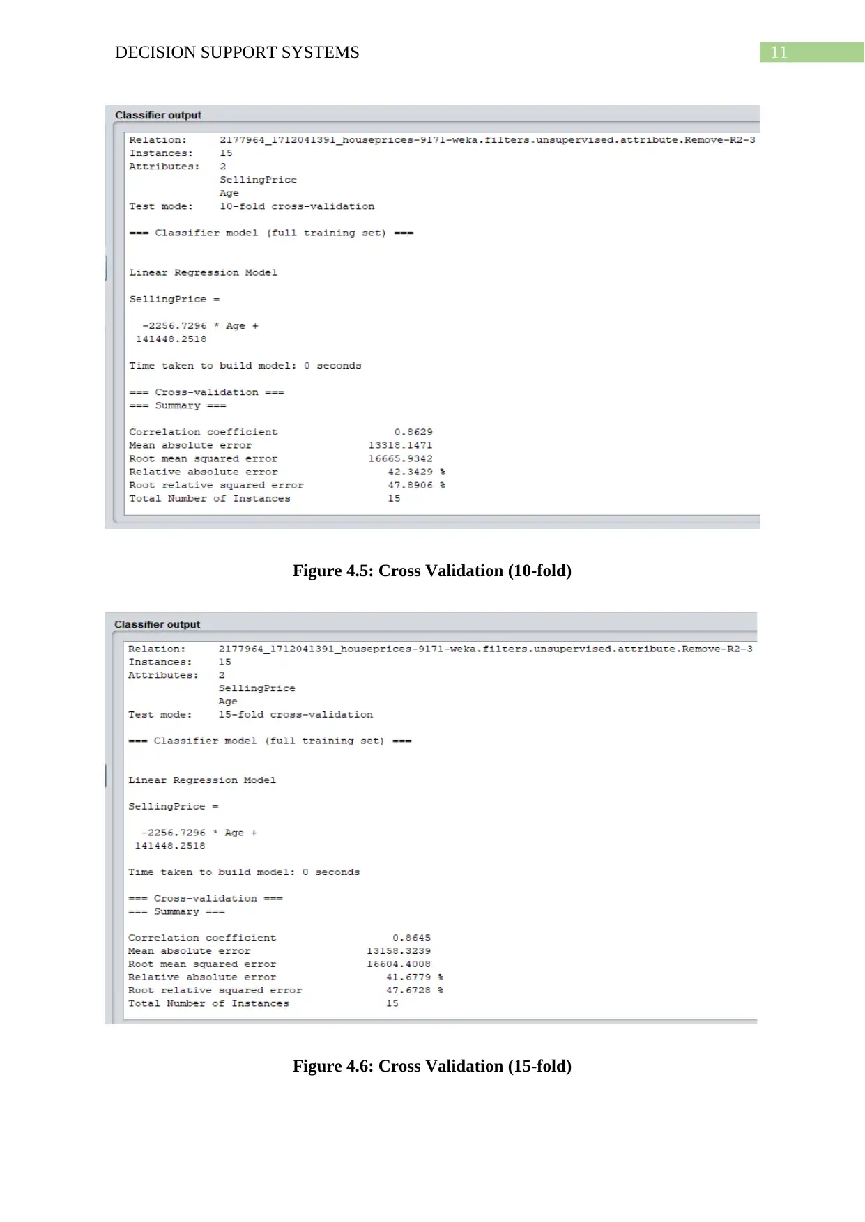
This project delves into Decision Support Systems (DSS), exploring various decision-making scenarios and analytical techniques. The assignment begins by analyzing strategic choices under uncertainty using payoff tables and expected value calculations. It then constructs and solves a linear programming model for optimal resource allocation. Further, it explores simulation techniques to evaluate inventory policies, comparing different reorder points and quantities. The project also applies regression analysis to predict house prices based on area, bedroom numbers, and age, evaluating model performance using cross-validation. Additionally, it employs a Multilayer Perceptron (MLP) model to predict house prices, comparing its accuracy with the regression model. The final section focuses on classification models, using logistic regression and Naive Bayes to predict bank account openings, including confusion matrices, ROC curves, and lift charts to assess model performance.

Running head: DECISION SUPPORT SYSTEMS
Decision Support Systems
Name of the Student
Name of the University
Author Note

1DECISION SUPPORT SYSTEMS
Table of Contents
Answer 1....................................................................................................................................2
Answer 2....................................................................................................................................4
Answer 3....................................................................................................................................6
Answer 4....................................................................................................................................6
Part 1......................................................................................................................................6
Part 2......................................................................................................................................7
Answer 5....................................................................................................................................9
Answer 6..................................................................................................................................10
Task 1...................................................................................................................................10
Task 2...................................................................................................................................12
Conclusion............................................................................................................................14

2DECISION SUPPORT SYSTEMS
Answer 1
There lies different opportunities for acquiring profit as well as loss in the concerned
business by Ilya and Gregor, which in turn depend on the set of three probable strategies
which yield different results in the favourable market and in the unfavourable market.
Strategy 1 involves Gregor and Ilya renting a considerably costly office in the location near
their probable customers. On the other hand, under Strategy 2, they can rent a comparatively
cheaper office in the neighbouring suburb region and the last strategy is the strategy of not at
all opening any business venture.
The outcomes of these strategies can be seen from the following table:
Table 1.1 Estimated Pay-Off (Positive or Negative) of the three strategies in different
markets
a. Strategy options for Ilya
Table 1.2: Ilya’s Strategy
As can be seen from the above, Ilya being a risk loving and optimist personnel is
eager to opt for maximum risk to get greater benefits. Keeping this into account the optimum
strategy in the perception of Ilya is that of Strategy 1, as here, both the risks as well as level
of expected profits are maximum.

3DECISION SUPPORT SYSTEMS
b. Strategy option for Gregor
Table 1.3 Gregor’s Strategy
Gregor being more conservative and risk averse than that of Ilya, the optimum
strategy of the same is the one with maximum profit along with minimum risk. Thus, Gregor
will choose the third strategy as the loss is minimum in the concerned strategy.
c. As can be seen from the concern problem, the probability of the market to be favourable
for the business is 0.55 while the probability of the same to be non-favourable is 0.45. Thus,
the expected pay-offs of each of the concerned strategies, in this situation, can be compared
with the help of the following table:
Table 1.4: Expected pay-offs of the different strategies
As is evident from the above numbers, the expected profit is comparatively highest in
case of the second strategy, which in turn indicates to the fact that the second strategy of
getting an office in the cheaper suburbs will be chosen.
d. If the probability of the presence of a favourable market is not fixed at 0.55 and instead
varies between range of 0 to 1, then according to the different values of the probability of the

4DECISION SUPPORT SYSTEMS
same the expected pay-offs or returns from the concerned market can be seen from the
following figure:
Figure 1: Expected pay-offs of different strategies when probability varies between 0
and 1
e. i. The probability range in which the first strategy can be chosen is 0.67≤P≤1
ii. The probability range in which the second strategy can be chosen is 0.29≤P≤0.66
iii. The probability range in which the third strategy can be chosen is 0≤P≤0.28
Answer 2
From the concerned problem, the linear programming model can be constructed as below:
Min (Z) = 960(TV) + 480 (Radio) + 600(Billboards) + 120 (Newspaper)
Subject to:
TV≤10
Radio≤10

5DECISION SUPPORT SYSTEMS
Billboards≤10
Newspaper≤10
TV≥6
Radio≥6
TV + Radio≥6
960(TV) – 600(Billboards) – 120(Newspaper)≥0
960(TV) + 480(Radios) + 600(Billboards) + 120(Newspapers)≤14000
Non-negativity constraints: TV≥0, Radios≥0, Newspaper≥0, Billboards≥0
The solution of the above problem can be seen as follows:
a. Thus, the maximum number of person Jim can reach within his weekly budget of 14,000
is:
= (6*36000) + (6*26500) +(8*30000) = 615000.

6DECISION SUPPORT SYSTEMS
b. To achieve the desired result Jim should post 6 ads on TV, 6 ads on Radio and 8 ads on the
billboards.
Answer 3
a. From the simulation result it can be seen that in the concerned scenario of Max, the best
case for least cost for the inventory policy is $49,000 and the worst case of highest cost for
the inventory policy is $63,020. Thus, the average cost of the concerned policy which will be
incurred by Max, taking into consideration, reorder point 5 and quantity 5 is of amount
$56,530.
b. i) In case of the reorder point being 3 and the reordering quantity being 3, the minimum
cost which has to be incurred by Max is $29,760 while the maximum cost of the same is
$40,260. The average cost incurred in this respect is $37,362.
b. ii) Taking into consideration the reward point 7 and the reordering quantity 7, the lowest
cost is $81,840 and that of the highest cost is that of $94,380, the average cost being $90,044.
c. Thus, it can be asserted clearly that in case of the reordering point 3 and reordering
quantity 3, the maximum cost for the inventory policy is lesser than even the minimum cost
which is incurred for the same in the case of reordering point 7 and reordering quantity 7,
which in turn implies that the former reordering point and quantity (3) is better than the latter
(7), thereby indicating that the former is a better option for the concerned business than the
latter.
Answer 4
Part 1
By taking area as the independent variable, the predicted selling prices for the house
can be seen as follows:

7DECISION SUPPORT SYSTEMS
Predicted Price = -34301.5987 + [62.96*(Area)]
For the concerned model, the coefficient of determination = (0.7952^2) = 0.6323.
This in turn shows that around 62.23% of the dynamics or variability of the price of the house
can be explained by the independent variable (Area) of the same.
Figure 4.1: Cross Validation (10-fold)

8DECISION SUPPORT SYSTEMS
Figure 4.2: Cross Validation (15-fold)
From 4.1 and 4.1 it can be seen that the training errors like relative absolute and the root
relative squared error are lower in 15-fold cross validation than in 10-fold cross validation.
Therefore, when Area is equal to 2000 square ft, the selling price of the same is as follows:
Price = -34301.5987 + (62.96*2000) = 91618.4
Now, considering bedrooms as the independent variable, the predicted selling price of
the concerned house is as follows:
Predicted Price = 648.6487 + [35168.9189*(Bedroom numbers)]
For this model, the determination coefficient = (0.5047^2) = 0.2547, which in turn
implies that nearly 25.47% of the variations in the price of the house can be explained by the
bedroom numbers present in the house.

9DECISION SUPPORT SYSTEMS
Thus, when the number of bedrooms in the house is 3,
Price = 648.6487 + [35168.9189*3] = 106155
Figure 4.3: Cross Validation (10-fold)

10DECISION SUPPORT SYSTEMS
Figure 4.4: Cross Validation (15-fold)
If age is considered to be the independent variable in the concerned problem, then,
Expected Price = 141448.2518 + [-2256.7296*(Age)]
The coefficient of determination being (0.8629^2) = 0.7446, nearly 74.46% of the selling
price variability of the house can be explained by the age of the same. Thus, when the age is
24 years,
Price = 141448.2518 + [-2256.7296*24] = 87286.7.

11DECISION SUPPORT SYSTEMS
Figure 4.5: Cross Validation (10-fold)
Figure 4.6: Cross Validation (15-fold)