University Decision Support Tools, Business Development Analysis

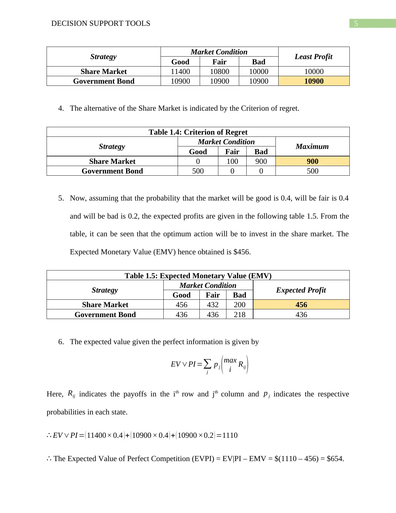
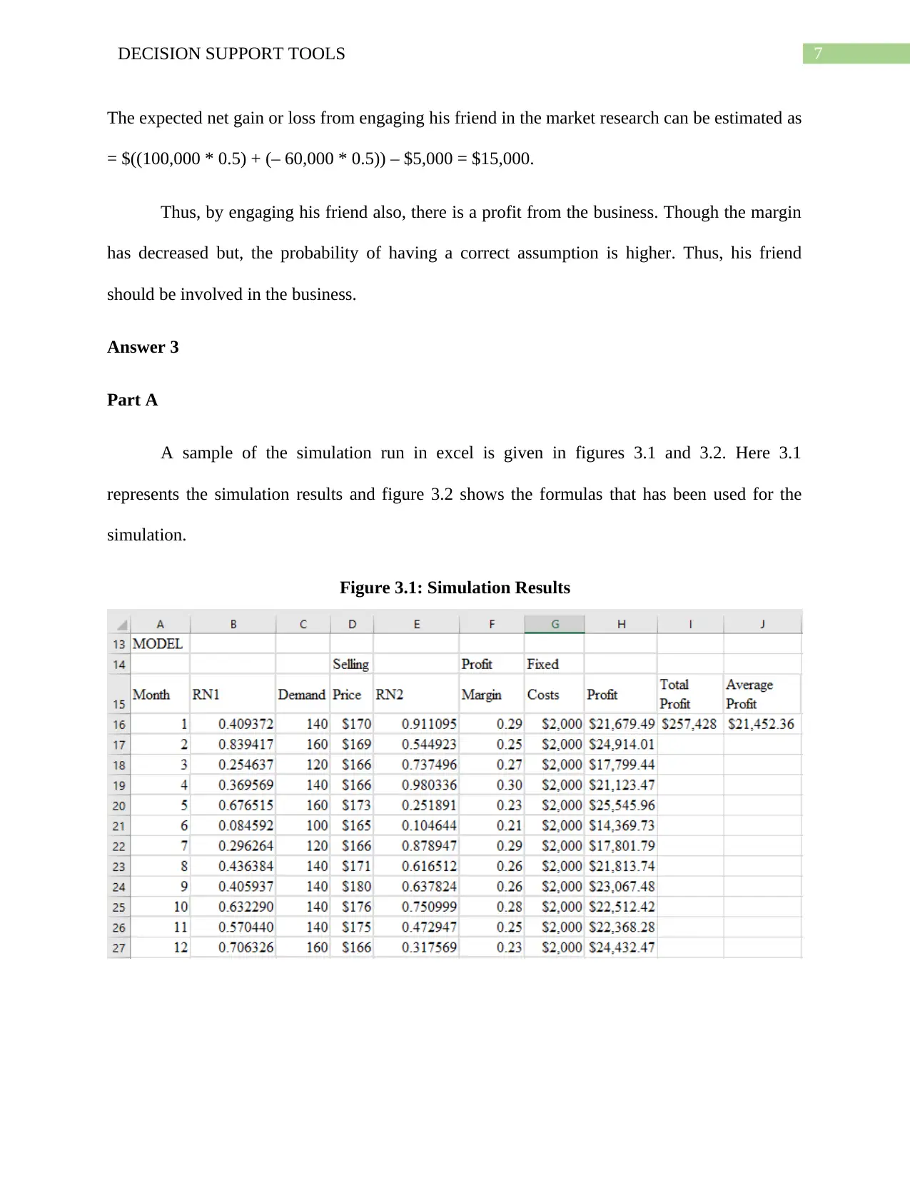
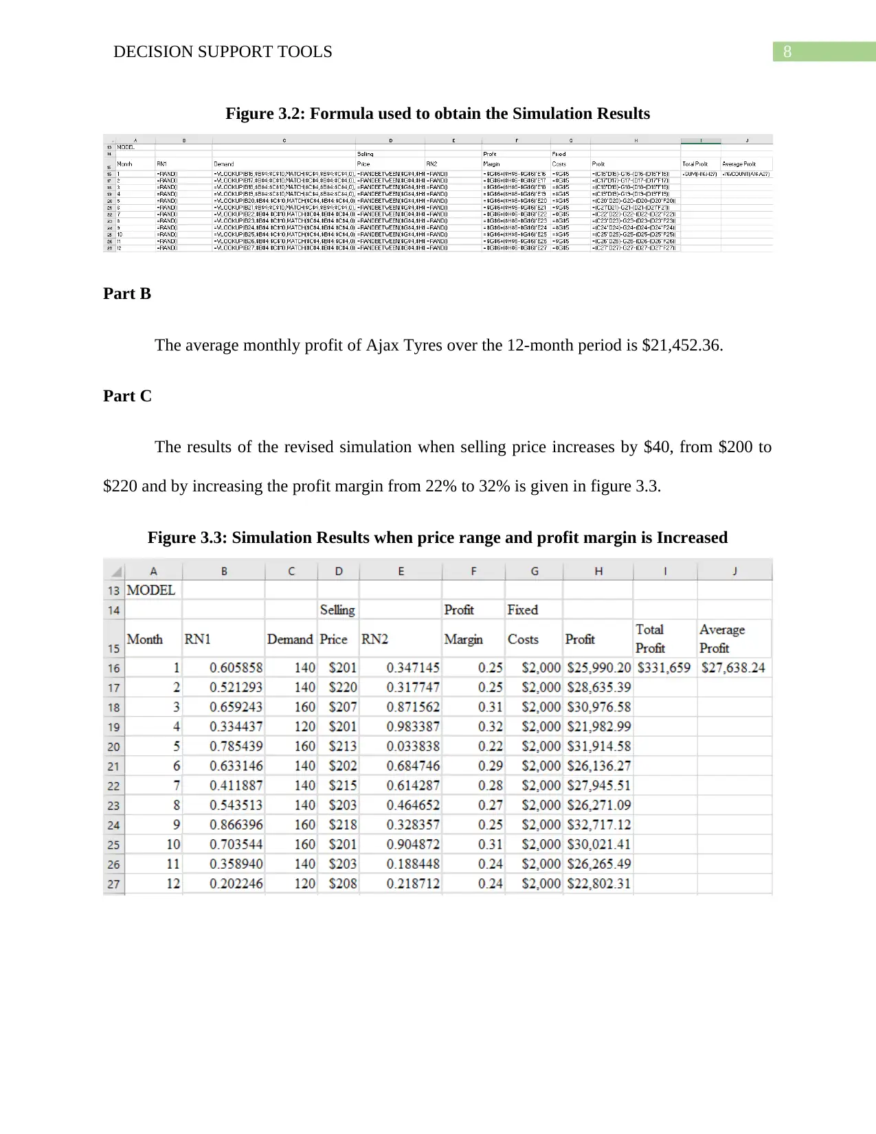
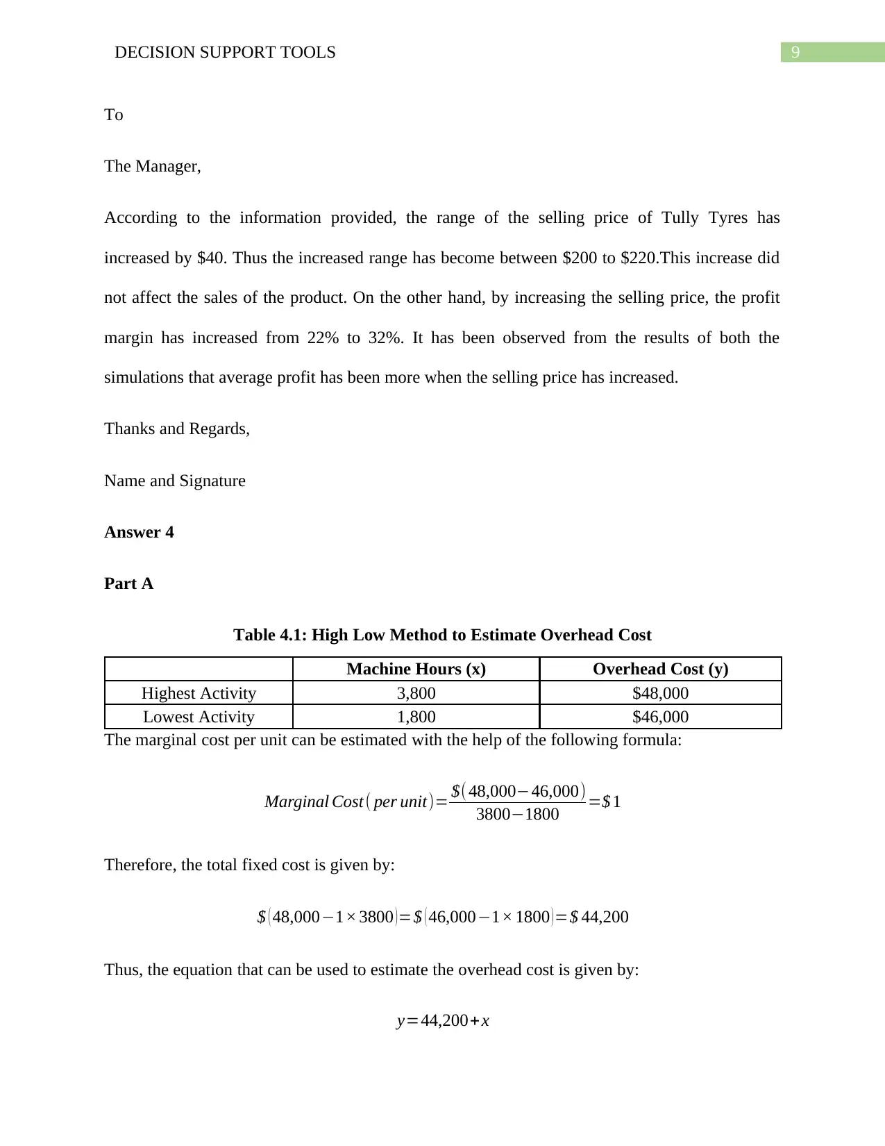
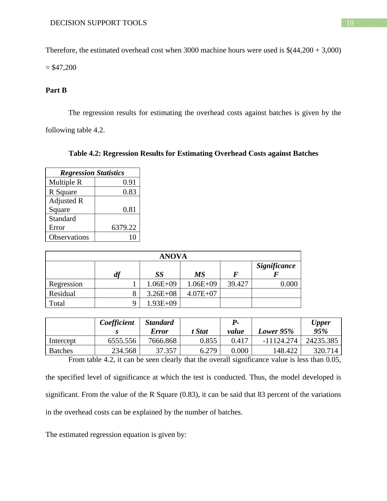
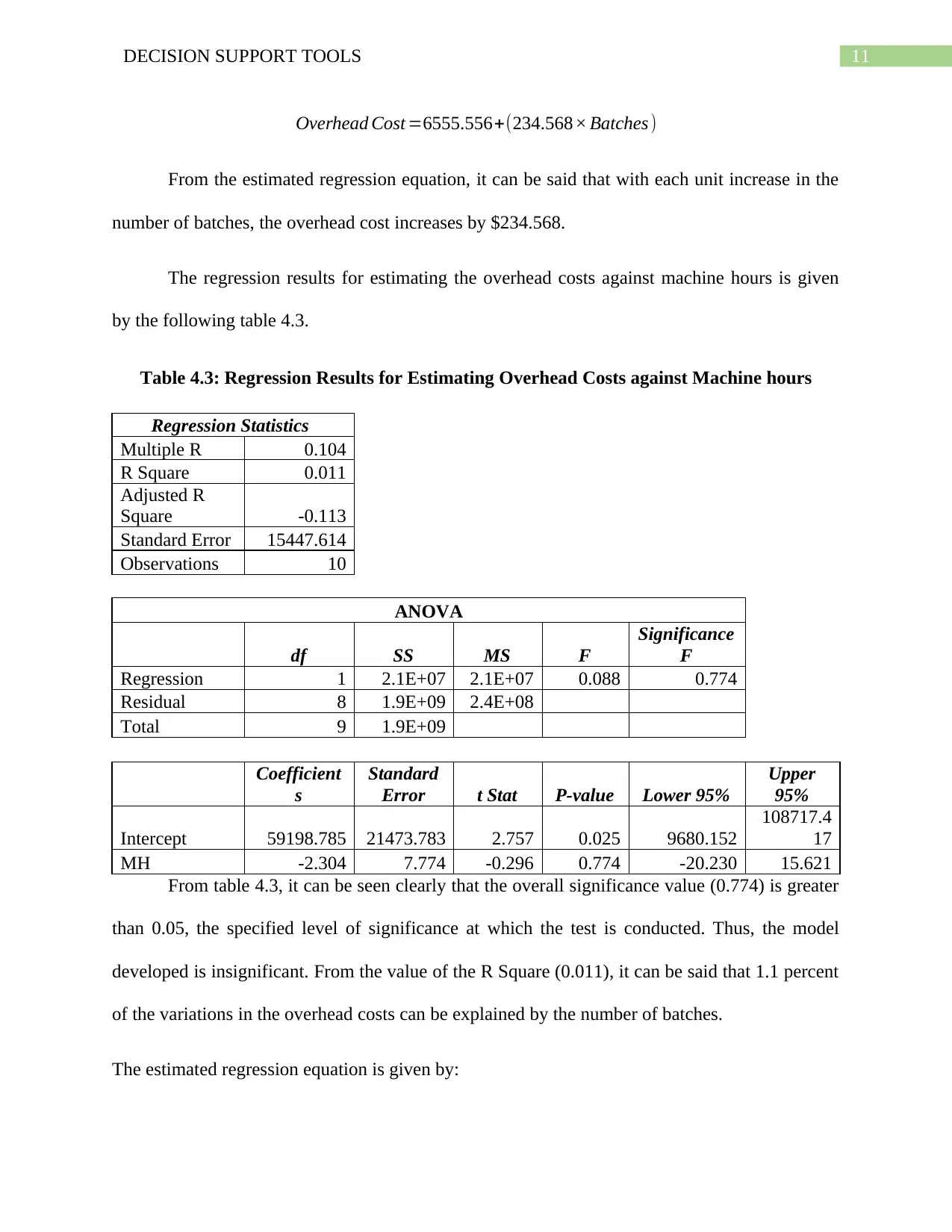
This assignment solution delves into the realm of decision support tools, providing comprehensive analyses of various business scenarios. It begins by exploring the concept of utility, outlining methods for its assessment and application in decision-making. The solution then presents a case study involving an investment decision, evaluating different strategies using decision matrices, optimist and pessimist approaches, and the criterion of regret. Furthermore, it incorporates expected monetary value calculations and the expected value of perfect information. The assignment proceeds to a scenario concerning a new product launch, analyzing expected returns under varying market conditions and incorporating the use of a friend's market predictions. The solution also includes a simulation analysis, showcasing the impact of different variables, such as selling price and profit margin, on business outcomes. Finally, it delves into cost estimation techniques, applying high-low methods and regression analysis to determine overhead costs based on machine hours and number of batches. The assignment provides detailed calculations, tables, and interpretations to support the findings, providing a comprehensive understanding of decision support tools and their application in business settings.

Running Head: DECISION SUPPORT TOOLS
Decision Support Tools
Name of the Student
Name of the University
Author Note

1DECISION SUPPORT TOOLS
Table of Contents
Answer 1..........................................................................................................................................3
Part A...........................................................................................................................................3
Part B...........................................................................................................................................4
Answer 2..........................................................................................................................................6
Part A...........................................................................................................................................6
Part B...........................................................................................................................................6
Part C...........................................................................................................................................6
Part D...........................................................................................................................................6
Answer 3..........................................................................................................................................7
Part A...........................................................................................................................................7
Part B...........................................................................................................................................8
Part C...........................................................................................................................................8
Answer 4..........................................................................................................................................9
Part A...........................................................................................................................................9
Part B.........................................................................................................................................10
Part C.........................................................................................................................................13
Part D.........................................................................................................................................13
Answer 5........................................................................................................................................13
Part A.........................................................................................................................................13

2DECISION SUPPORT TOOLS
Part B.........................................................................................................................................14
Part C.........................................................................................................................................14
Part D.........................................................................................................................................14
References......................................................................................................................................16

3DECISION SUPPORT TOOLS
Answer 1
Part A
Utility is the level of satisfaction that an individual enjoys from a consuming certain units
of a commodity. There are several methods of assessing a utility function. The first step in
assessing utility function is structure the decision problem. This is followed by development an
appropriate measurement scale for evaluating the attributes. The decision maker then needs to
acquaint with different aspect related to assessment procedure. The second step is to identify the
special characteristics relevant to the typical utility function (Li, 2014). Quantitative restrictions
then need to specify for utility function of the decision maker in terms of comparison of different
gambles for attributes under consideration. For assessment of final utility, a utility function is to
be specified accomplishing the all the earlier mentioned characteristics.
Standard gamble is common way of assessing utility. The best outcome in a standard
gamble is assigned with a utility of 1. The worst outcome in the gamble has an assigned utility of
0. The intermediate outcomes are then selected between the best and worst outcome. Decision
maker then needs to make a choice between intermediary outcomes obtained for sure and gamble
that involve best and worst outcomes. The associated probability for which the decision maker is
indifferent between utility obtained from intermediary outcomes and that of a gamble is
determined (Kuspinar, Pickard & Mayo, 2016). The determined probability then is the utility
associated to the intermediate outcomes. The process continues unless utility values of all
possible economic scenarios are determined. The values of the utility are then plotted on a curve
called the utility curve.

4DECISION SUPPORT TOOLS
Part B
Allan Barnes decides to invest $10,000 in a government bond or share market. The interest rate
for the bond is 9% whereas in the share market, when the market is good, fair or bad, the interest
rates vary from 14%, 8% and 0% respectively.
1. The decision matrix showing all the possible strategies is given in the following table:
Table 1.1: Decision Matrix showing all possible strategies
Strategy Market Condition
Good Fair Bad
Share Market 11400 10800 10000
Government Bond 19000 19000 19000
2. An optimist always hopes for the best to happen. Thus, an optimist would choose
the strategy that will be giving the maximum return. It can be seen from table 1.2 that, the
maximum profit can be earned from the Share Market. Thus, an optimist would choose to
invest in the share market.
Table 1.2: Optimist Approach
Strategy Market Condition Best Profit
Good Fair Bad
Share Market 11400 10800 10000 11400
Government Bond 10900 10900 10900 10900
3. A pessimist will always imagine the worst possible scenario to happen. Thus, a pessimist
would choose a strategy in which he can have the maximum profit with the minimum
risk. Thus, according to a pessimist the best investment scheme would be in the
Government Bond as it can earn the maximum return even when the market is bad or
poor.
Table 1.3: Pessimist Approach

5DECISION SUPPORT TOOLS
Strategy Market Condition Least Profit
Good Fair Bad
Share Market 11400 10800 10000 10000
Government Bond 10900 10900 10900 10900
4. The alternative of the Share Market is indicated by the Criterion of regret.
Table 1.4: Criterion of Regret
Strategy Market Condition Maximum
Good Fair Bad
Share Market 0 100 900 900
Government Bond 500 0 0 500
5. Now, assuming that the probability that the market will be good is 0.4, will be fair is 0.4
and will be bad is 0.2, the expected profits are given in the following table 1.5. From the
table, it can be seen that the optimum action will be to invest in the share market. The
Expected Monetary Value (EMV) hence obtained is $456.
Table 1.5: Expected Monetary Value (EMV)
Strategy Market Condition Expected Profit
Good Fair Bad
Share Market 456 432 200 456
Government Bond 436 436 218 436
6. The expected value given the perfect information is given by
EV ∨PI =∑
j
p j ( max
i Rij )
Here, Rij indicates the payoffs in the ith row and jth column and p j indicates the respective
probabilities in each state.
∴ EV ∨PI = ( 11400× 0.4 )+ (10900 × 0.4 ) + ( 10900 ×0.2 ) =1110
∴ The Expected Value of Perfect Competition (EVPI) = EV|PI – EMV = $(1110 – 456) = $654.

6DECISION SUPPORT TOOLS
Answer 2
It has been the thought by Jim that he will be launching a new variety of men’s razor.
Return in favorable market = $100,000
Return in unfavorable market = – $60,000
The probability that the market is favorable = 0.5
Therefore, the probability that the market is unfavorable = (1 – 0.5) = 0.5.
Part A
The expected return that can be earned from the market = $((100,000 * 0.5) + (– 60,000 * 0.5)) =
$20,000.
Therefore, on an average, he will incur a profit by producing the product in the market.
Therefore, he should produce the product in the market.
Part B
Based on the track record of his friend, the probability that the market is favorable = (0.5 * 0.7) +
(0.5 * 0.3) = 0.5 and the probability that the market is unfavorable = (0.5 * 0.2) + (0.5 * 0.8) =
0.5
Part C
The posterior probability of a good market given that his friend has provided an unfavorable
market prediction = (0.3 * 0.5) = 0.15.
Part D

7DECISION SUPPORT TOOLS
The expected net gain or loss from engaging his friend in the market research can be estimated as
= $((100,000 * 0.5) + (– 60,000 * 0.5)) – $5,000 = $15,000.
Thus, by engaging his friend also, there is a profit from the business. Though the margin
has decreased but, the probability of having a correct assumption is higher. Thus, his friend
should be involved in the business.
Answer 3
Part A
A sample of the simulation run in excel is given in figures 3.1 and 3.2. Here 3.1
represents the simulation results and figure 3.2 shows the formulas that has been used for the
simulation.
Figure 3.1: Simulation Results

8DECISION SUPPORT TOOLS
Figure 3.2: Formula used to obtain the Simulation Results
Part B
The average monthly profit of Ajax Tyres over the 12-month period is $21,452.36.
Part C
The results of the revised simulation when selling price increases by $40, from $200 to
$220 and by increasing the profit margin from 22% to 32% is given in figure 3.3.
Figure 3.3: Simulation Results when price range and profit margin is Increased

9DECISION SUPPORT TOOLS
To
The Manager,
According to the information provided, the range of the selling price of Tully Tyres has
increased by $40. Thus the increased range has become between $200 to $220.This increase did
not affect the sales of the product. On the other hand, by increasing the selling price, the profit
margin has increased from 22% to 32%. It has been observed from the results of both the
simulations that average profit has been more when the selling price has increased.
Thanks and Regards,
Name and Signature
Answer 4
Part A
Table 4.1: High Low Method to Estimate Overhead Cost
Machine Hours (x) Overhead Cost (y)
Highest Activity 3,800 $48,000
Lowest Activity 1,800 $46,000
The marginal cost per unit can be estimated with the help of the following formula:
Marginal Cost ( per unit)= $( 48,000−46,000)
3800−1800 =$ 1
Therefore, the total fixed cost is given by:
$ ( 48,000−1× 3800 ) =$ ( 46,000−1× 1800 ) =$ 44,200
Thus, the equation that can be used to estimate the overhead cost is given by:
y=44,200+x

10DECISION SUPPORT TOOLS
Therefore, the estimated overhead cost when 3000 machine hours were used is $(44,200 + 3,000)
= $47,200
Part B
The regression results for estimating the overhead costs against batches is given by the
following table 4.2.
Table 4.2: Regression Results for Estimating Overhead Costs against Batches
Regression Statistics
Multiple R 0.91
R Square 0.83
Adjusted R
Square 0.81
Standard
Error 6379.22
Observations 10
ANOVA
df SS MS F
Significance
F
Regression 1 1.06E+09 1.06E+09 39.427 0.000
Residual 8 3.26E+08 4.07E+07
Total 9 1.93E+09
Coefficient
s
Standard
Error t Stat
P-
value Lower 95%
Upper
95%
Intercept 6555.556 7666.868 0.855 0.417 -11124.274 24235.385
Batches 234.568 37.357 6.279 0.000 148.422 320.714
From table 4.2, it can be seen clearly that the overall significance value is less than 0.05,
the specified level of significance at which the test is conducted. Thus, the model developed is
significant. From the value of the R Square (0.83), it can be said that 83 percent of the variations
in the overhead costs can be explained by the number of batches.
The estimated regression equation is given by:

11DECISION SUPPORT TOOLS
Overhead Cost =6555.556+(234.568× Batches)
From the estimated regression equation, it can be said that with each unit increase in the
number of batches, the overhead cost increases by $234.568.
The regression results for estimating the overhead costs against machine hours is given
by the following table 4.3.
Table 4.3: Regression Results for Estimating Overhead Costs against Machine hours
Regression Statistics
Multiple R 0.104
R Square 0.011
Adjusted R
Square -0.113
Standard Error 15447.614
Observations 10
ANOVA
df SS MS F
Significance
F
Regression 1 2.1E+07 2.1E+07 0.088 0.774
Residual 8 1.9E+09 2.4E+08
Total 9 1.9E+09
Coefficient
s
Standard
Error t Stat P-value Lower 95%
Upper
95%
Intercept 59198.785 21473.783 2.757 0.025 9680.152
108717.4
17
MH -2.304 7.774 -0.296 0.774 -20.230 15.621
From table 4.3, it can be seen clearly that the overall significance value (0.774) is greater
than 0.05, the specified level of significance at which the test is conducted. Thus, the model
developed is insignificant. From the value of the R Square (0.011), it can be said that 1.1 percent
of the variations in the overhead costs can be explained by the number of batches.
The estimated regression equation is given by:

12DECISION SUPPORT TOOLS
Overhead Cost =59198.785−(2.304 × Machine Hours)
From the estimated regression equation, it can be said that with each unit increase in the
machine hours, the overhead cost decreases by $2.304.
The regression results for estimating the overhead costs against machine hours is given
by the following table 4.4.
Table 4.4: Regression Results for Estimating Overhead Costs against Machine hours and
Number of Batches
Regression Statistics
Multiple R 0.913
R Square 0.833
Adjusted R
Square 0.785
Standard
Error 6783.922
Observations 10
ANOVA
df SS MS F
Significance
F
Regression 2 1.6E+09 8.0E+08 17.468 0.002
Residual 7 3.2E+08 4.6E+07
Total 9 1.9E+09
Coefficients
Standard
Error t Stat
P-
value Lower 95%
Upper
95%
Intercept 9205.658 12704.918 0.725 0.492 -20836.700 39248.016
MH -0.931 3.422 -0.272 0.793 -9.022 7.161
Batches 233.827 39.820 5.872 0.001 139.667 327.987
From table 4.4, it can be seen clearly that the overall significance value (0.002) is less
than 0.05, the specified level of significance at which the test is conducted. Thus, the model
developed is significant. From the value of the R Square (0.833), it can be said that 83.3 percent
of the variations in the overhead costs can be explained by the number of batches and overhead

13DECISION SUPPORT TOOLS
cost. Moreover, it can be seen from the model that the variable Machine hours is insignificant but
the variable number of batches is significant.
The estimated regression equation is given by:
Overhead Cost =9205.658− ( 0.931× Machine Hours ) +(233.827 × Batches)
From the estimated regression equation, it can be said that with each unit increase in the
machine hours, the overhead cost decreases by $0.931 and with each unit increase in batches, the
overhead cost increases by $233.827.
Part C
From the regression models developed, it can be seen clearly that for the regression
model 1 and 3, the value of r Square are the same, but the value of the adjusted R Square is
higher for the first model. Thus, it can be said that Batches is a better estimator of overhead cost
than the overall model.
Part D
The estimated overhead cost in a month when 150 batches of the product has been
produced is:
Overhead Cost =6555.556+ ( 234.568 ×150 ) =$ 41,740.74
Answer 5
Part A
For product A, the sales price per unit is $12 and the variable cost per unit is $8. Thus,
the contribution margin is $ (12 – 8) = $4.

14DECISION SUPPORT TOOLS
Similarly, for product B, the sales price per unit is $15 and the variable cost per unit is
$10. Thus, the contribution margin is $ (15 – 10) = $5.
Part B
If the manufacturer specializes only in Product B, then the manufacturer needs to sell
(5000 / 5) units = 1000 units.
Part C
If the manufacturer specializes only in Product A, then the manufacturer needs to sell
(5000 / 4) units = 1250 units.
Part D
If the manufacturer decides to manufacture both the products A and B, in the ratio of 3:1
respectively,
(i) In order to earn a profit of $3,500 before tax for the month, the number of products of A
that has to be sold is 1333 and the number of products of B that has to be sold is 667. The
necessary calculations are shown in table 5.1.
Table 5.1
Product A B Total
Sales Unit 3 1 4
Sales price $36 $15 $51
Variable cost $24 $10 $34
Total fixed costs $5,000
Total Contribution $12 $5 $17
Weighted average Contribution $4
Targeted Profit (Before Tax) $3,500
Targeted Sales Volume 1333 667 2000

15DECISION SUPPORT TOOLS
(ii) In order to earn a profit of $8,400 after tax for the month, the number of products of A
that has to be sold is 855 and the number of products of B that has to be sold is 428. The
necessary calculations are shown in table 5.2.
Table 5.2
Product A B Total
Sales Unit 3 1 4
Sales price $72 $15 $87
Variable cost $24 $10 $34
Total fixed costs $5,000
Total Contribution $48 $5 $53
Weighted average Contribution $13
Targeted Profit (After Tax) $8,400
Tax Rate 30%
Targeted Profit (Before Tax) 12000
Targeted Sales Volume 855 428 1283

16DECISION SUPPORT TOOLS
References
Kuspinar, A., Pickard, S., & Mayo, N. E. (2016). Developing a valuation function for the
preference-based multiple sclerosis index: comparison of standard gamble and rating
scale. PloS one, 11(4), e0151905.
Li, W. (2014). Risk assessment of power systems: models, methods, and applications. John
Wiley & Sons.