Decision Support Tools: Statistical Analysis and Decision Making

This document presents a comprehensive solution to an assignment on decision support tools. The assignment covers several key concepts, including the calculation of expected value and probabilities using discrete probability distributions, as demonstrated through examples of daily bread sales. It explores the calculation of probabilities related to product quality from multiple machines, and applies the normal distribution to calculate probabilities related to apple sales. The solution also addresses confidence intervals and hypothesis testing, computing a 95% confidence interval and performing a hypothesis test to compare the average age of laid-off employees with the average age of current employees. The document includes detailed calculations, interpretations, and references, providing a thorough understanding of the application of statistical methods in decision-making processes.

DECISION SUPPORT TOOLS
[Document subtitle]
[DATE]

Question 1
(a)The expected value is the average value that may be derived for an event whose outcomes
are probabilistic. Thus, it highlights an average estimation of the output based on the
respective probabilities associated with the outcomes. For a discrete probability
distribution, this may be computed by finding the respective probabilities of various
outcomes. Then the sum of the product of outcome and their respective probability is
computed for all the possible outcomes (Eriksson & Kovalainen, 2015).
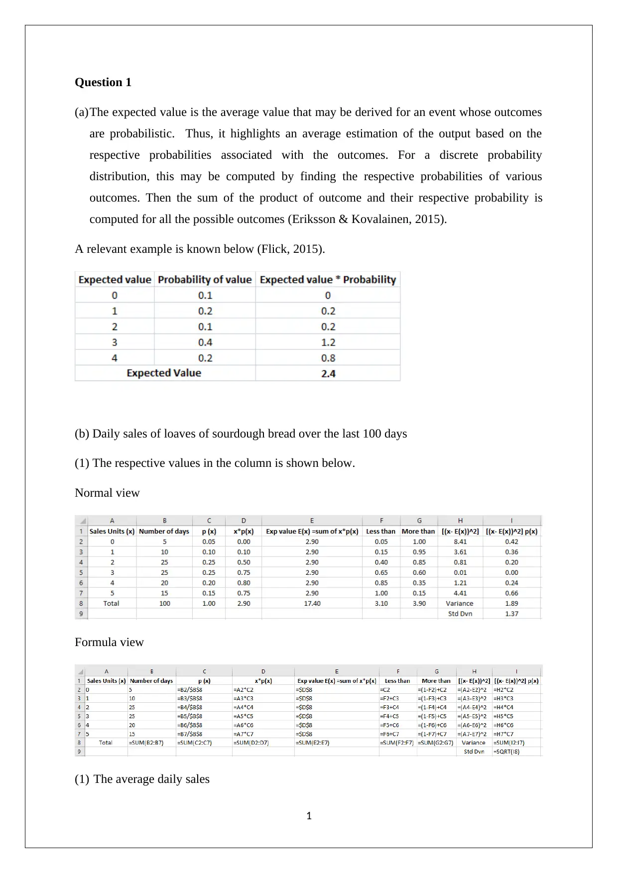
A relevant example is known below (Flick, 2015).
(b) Daily sales of loaves of sourdough bread over the last 100 days
(1) The respective values in the column is shown below.
Normal view
Formula view
(1) The average daily sales
1

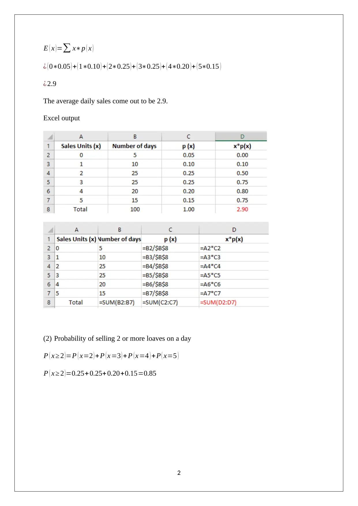
E ( x ) =∑ x∗p ( x )
¿ ( 0∗0.05 ) + ( 1∗0.10 ) + ( 2∗0.25 )+ ( 3∗0.25 )+ ( 4∗0.20 )+ ( 5∗0.15 )
¿ 2.9
The average daily sales come out to be 2.9.
Excel output
(2) Probability of selling 2 or more loaves on a day
P ( x ≥ 2 )=P ( x=2 ) + P ( x =3 ) + P ( x =4 ) +P ( x=5 )
P ( x ≥ 2 )=0.25+0.25+ 0.20+0.15=0.85
2

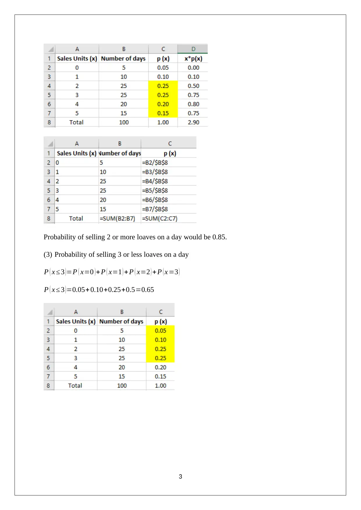
Probability of selling 2 or more loaves on a day would be 0.85.
(3) Probability of selling 3 or less loaves on a day
P ( x ≤ 3 ) =P ( x=0 ) + P ( x=1 ) + P ( x=2 ) + P ( x =3 )
P ( x ≤ 3 )=0.05+0.10+0.25+0.5=0.65
3

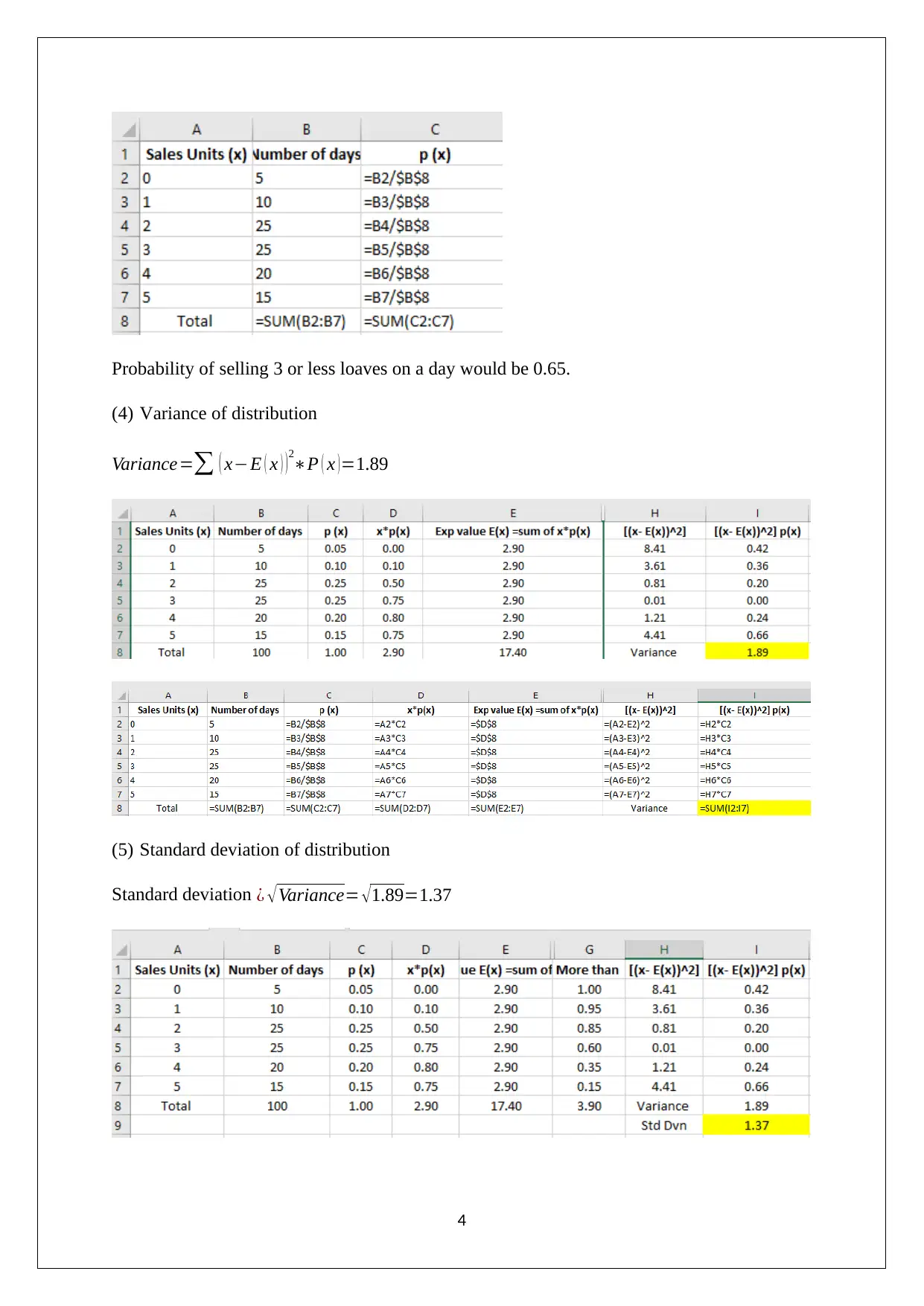
Probability of selling 3 or less loaves on a day would be 0.65.
(4) Variance of distribution
Variance=∑ ( x−E ( x ) )2
∗P ( x )=1.89
(5) Standard deviation of distribution
Standard deviation ¿ √Variance= √1.89=1.37
4

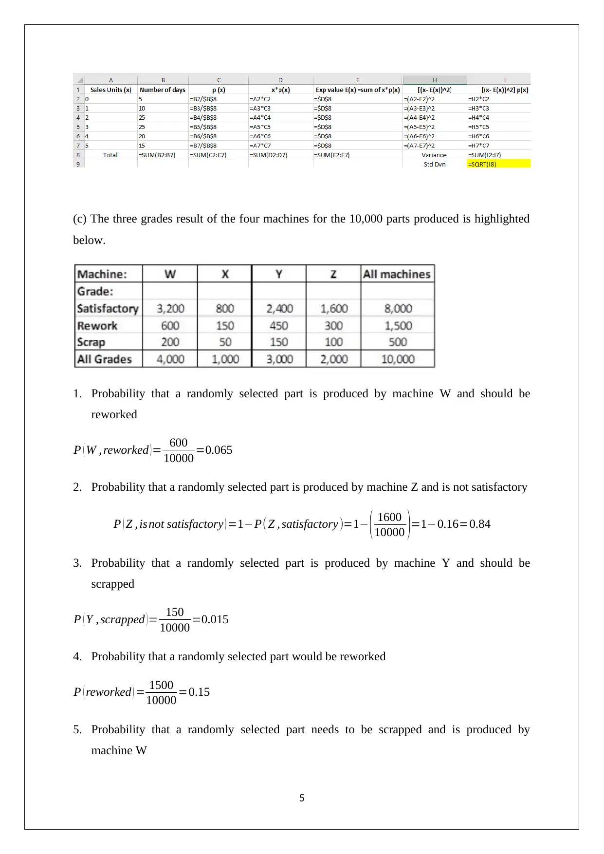
(c) The three grades result of the four machines for the 10,000 parts produced is highlighted
below.
1. Probability that a randomly selected part is produced by machine W and should be
reworked
P ( W , reworked )= 600
10000 =0.065
2. Probability that a randomly selected part is produced by machine Z and is not satisfactory
P ( Z , isnot satisfactory ) =1−P( Z , satisfactory )=1− ( 1600
10000 )=1−0.16=0.84
3. Probability that a randomly selected part is produced by machine Y and should be
scrapped
P ( Y , scrapped )= 150
10000 =0.015
4. Probability that a randomly selected part would be reworked
P ( reworked ) = 1500
10000 =0.15
5. Probability that a randomly selected part needs to be scrapped and is produced by
machine W
5

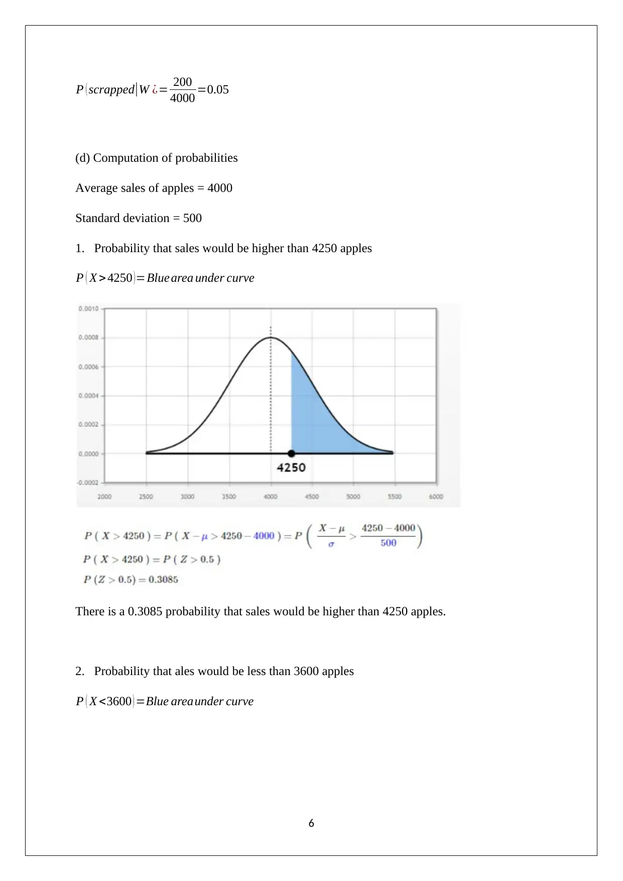
P ( scrapped|W ¿= 200
4000 =0.05
(d) Computation of probabilities
Average sales of apples = 4000
Standard deviation = 500
1. Probability that sales would be higher than 4250 apples
P ( X > 4250 )=Blue area under curve
There is a 0.3085 probability that sales would be higher than 4250 apples.
2. Probability that ales would be less than 3600 apples
P ( X <3600 ) =Blue areaunder curve
6

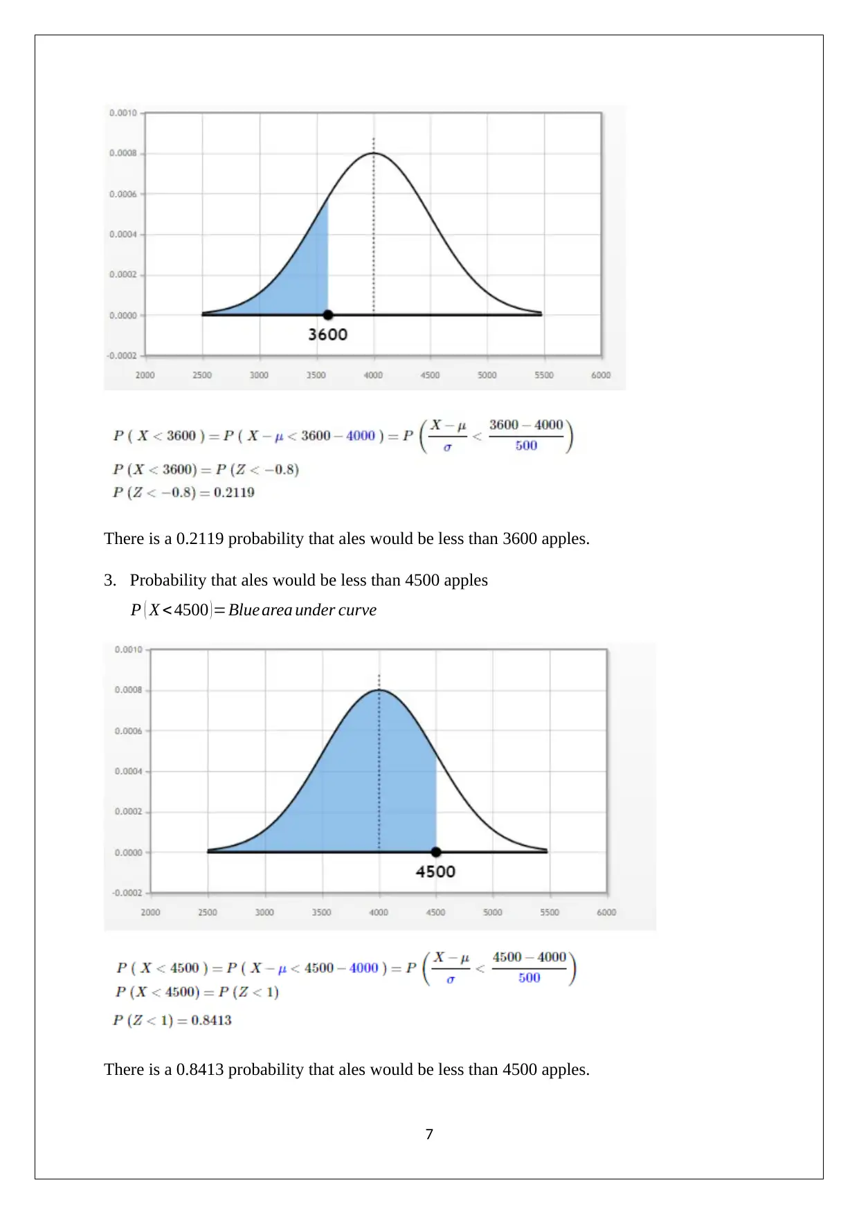
There is a 0.2119 probability that ales would be less than 3600 apples.
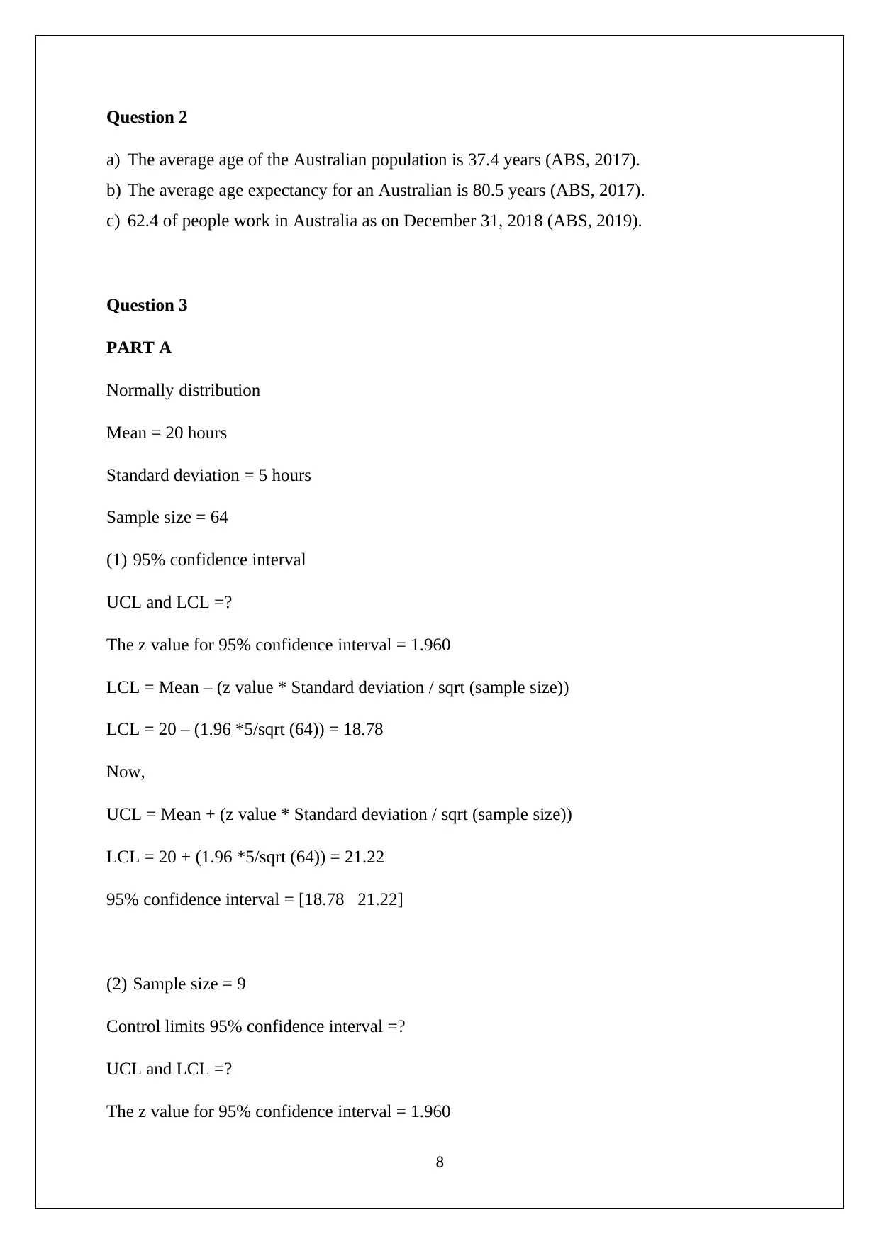
3. Probability that ales would be less than 4500 apples
P ( X < 4500 )=Blue area under curve
There is a 0.8413 probability that ales would be less than 4500 apples.
7

Question 2
a) The average age of the Australian population is 37.4 years (ABS, 2017).
b) The average age expectancy for an Australian is 80.5 years (ABS, 2017).
c) 62.4 of people work in Australia as on December 31, 2018 (ABS, 2019).
Question 3
PART A
Normally distribution
Mean = 20 hours
Standard deviation = 5 hours
Sample size = 64
(1) 95% confidence interval
UCL and LCL =?
The z value for 95% confidence interval = 1.960
LCL = Mean – (z value * Standard deviation / sqrt (sample size))
LCL = 20 – (1.96 *5/sqrt (64)) = 18.78
Now,
UCL = Mean + (z value * Standard deviation / sqrt (sample size))
LCL = 20 + (1.96 *5/sqrt (64)) = 21.22
95% confidence interval = [18.78 21.22]
(2) Sample size = 9
Control limits 95% confidence interval =?
UCL and LCL =?
The z value for 95% confidence interval = 1.960
8

LCL = Mean – (z value * Standard deviation / sqrt (sample size))
LCL = 20 – (1.96 *5/sqrt (9)) = 16.73
Now,
UCL = Mean + (z value * Standard deviation / sqrt (sample size))
LCL = 20 + (1.96 *5/sqrt (9)) = 23.27
95% confidence interval = [16.73 23.27]
PART B
Hypothesis testing
Mean age = 45
Number of employees = 49
Standard deviation = 10.8 years
Significance level = 0.05
(1) Null and alternative hypothesis
Null hypothesis H0: μ=42, The average age of laid off is same as the average age of the
employees.
Alternative hypothesis Ha: μ > 42, The average age of the laid off is higher than the average
age of the employees.
(2) Critical value of Z
The test statistics
z stat = x−μ
σ
√ n
= 45−4
10.8
√ 49
=1.944
9

It is a right tailed hypothesis testing and hence, the null hypothesis would only be rejected if
the computed z stat is higher than the critical value of z (Hillier, 2016).
For 5% significance level, the z critical value = z1−∝=z0.95 =1.6449
It can be seen from the above that null hypothesis would be rejected because computed z stat
(1.944) is higher than the critical value of z (1.6449). Thus, reject null hypothesis (Hastie,
Tibshirani & Friedman, 2014).
(3) Rejection region
z stat =1.944 (Computed)
z0.95=1.6449 (Critical value)
(4) Conclusion
As the null hypothesis has rejected and alternative hypothesis is accepted. Hence, it can be
said that the average age of the laid off is higher than the average employee age.
10

References
ABS (2019) 6202.0 - Labour Force, Australia, Jan 2019, Retrieved on March 20, 2019 from
http://www.abs.gov.au/ausstats/abs@.nsf/mf/6202.0
ABS (2017) 3101.0 - Australian Demographic Statistics, Jun 2017, Retrieved on March 20,
2019 from
https://www.abs.gov.au/AUSSTATS/abs@.nsf/featurearticlesbyCatalogue/
CCF53AA000E69954CA2582570013F5C6?OpenDocument
Eriksson, P. & Kovalainen, A. (2015). Quantitative methods in business research (3rded.).
London: Sage Publications.
Flick, U. (2015). Introducing research methodology: A beginner's guide to doing a research
project (4thed.). New York: Sage Publications.
Hastie, T., Tibshirani, R. & Friedman, J. (2016). The Elements of Statistical Learning
(4thed.). New York: Springer Publications.
Hillier, F. (2016).Introduction to Operations Research.(6thed.). New York: McGraw Hill
Publications.
11