Analyzing Business Problems with Decision Support Tools Report
VerifiedAdded on 2023/06/05
|17
|2620
|188
Report
AI Summary
This report provides a comprehensive analysis of business problem-solving using various decision support tools. It covers topics such as utility functions, decision matrices, expected monetary value (EMV), Bayesian probability revisions, and regression analysis. The report includes practical examples, such as investment decisions, profit maximization for Ajax Tyres, and overhead cost analysis. It also demonstrates how to determine break-even points using Excel's Solver tool. The analysis utilizes tools like decision matrices, regression models, and simulation to provide insights into optimizing business decisions under different market conditions. The document concludes with recommendations for effective implementation of the analyzed models, emphasizing the importance of market surveys and validation of assumptions. Desklib provides access to this and many other solved assignments.

[1]
Problem Solving by Decision Support Tools
Problem Solving by Decision Support Tools
Paraphrase This Document
Need a fresh take? Get an instant paraphrase of this document with our AI Paraphraser
[2]
Table of Contents
Answer 1:.....................................................................................................................................................3
Answer 2:.....................................................................................................................................................5
Answer 3:.....................................................................................................................................................7
Answer 4:...................................................................................................................................................11
Answer 5:...................................................................................................................................................14
References.................................................................................................................................................17
Table of Tables
Table 1: Decision Table for Investment Value for Three Different Market Scenarios.....................4
Table 2: Optimistic Decision Matrix........................................................................................................4
Table 3: Max-Min (Pessimistic) Decision...............................................................................................4
Table 4: Regret Decision Matrix.............................................................................................................4
Table 5: Decision Matrix for EMV with Probabilities............................................................................5
Table 6: EMV of Profit from Jerry’s predictions....................................................................................5
Table 7: Revised Probabilities by Bayesian Model..............................................................................5
Table 8: Posterior Probabilities of Sales................................................................................................6
Table 9: Net Expected Value under Favorable and Unfavorable Market Conditions......................6
Table 10: Expected Average Monthly Profit Model of Ajax Tyres......................................................7
Table 11: Expected Average Monthly Profit Model for Ajax Tyres – Excel Formula of Table 10
Calculations...............................................................................................................................................8
Table 12: New Expected Average Monthly Profit Model for Ajax Tyres............................................9
Table 13: Regression Model for Overhead Cost on Machine Hour.................................................11
Table 14: Regression Model for Overhead Cost on Batches...........................................................12
Table 15: Regression Model for Overhead Cost on Machine Hour and Batches..........................13
Table 16: Optimal Products Sold for Product B..................................................................................15
Table 17: Optimal Product Sold for Product A....................................................................................15
Table 18: Optimal Product Quantity for Simultaneous Production of Products A & B...................16
Table 19: Profit from Parallel Production of A & B after Tax Deduction..........................................17
[3]
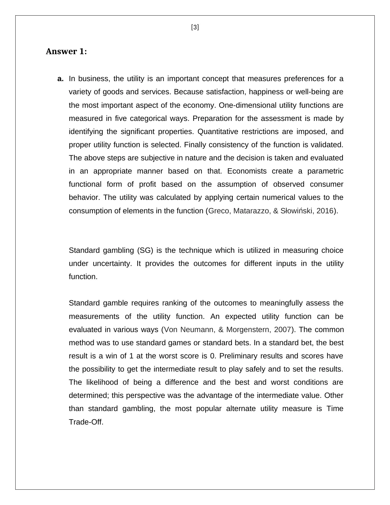
Answer 1:
a. In business, the utility is an important concept that measures preferences for a
variety of goods and services. Because satisfaction, happiness or well-being are
the most important aspect of the economy. One-dimensional utility functions are
measured in five categorical ways. Preparation for the assessment is made by
identifying the significant properties. Quantitative restrictions are imposed, and
proper utility function is selected. Finally consistency of the function is validated.
The above steps are subjective in nature and the decision is taken and evaluated
in an appropriate manner based on that. Economists create a parametric
functional form of profit based on the assumption of observed consumer
behavior. The utility was calculated by applying certain numerical values to the
consumption of elements in the function (Greco, Matarazzo, & Słowiński, 2016).
Standard gambling (SG) is the technique which is utilized in measuring choice
under uncertainty. It provides the outcomes for different inputs in the utility
function.
Standard gamble requires ranking of the outcomes to meaningfully assess the
measurements of the utility function. An expected utility function can be
evaluated in various ways (Von Neumann, & Morgenstern, 2007). The common
method was to use standard games or standard bets. In a standard bet, the best
result is a win of 1 at the worst score is 0. Preliminary results and scores have
the possibility to get the intermediate result to play safely and to set the results.
The likelihood of being a difference and the best and worst conditions are
determined; this perspective was the advantage of the intermediate value. Other
than standard gambling, the most popular alternate utility measure is Time
Trade-Off.
⊘ This is a preview!⊘
Do you want full access?
Subscribe today to unlock all pages.
Trusted by 1+ million students worldwide
[4]
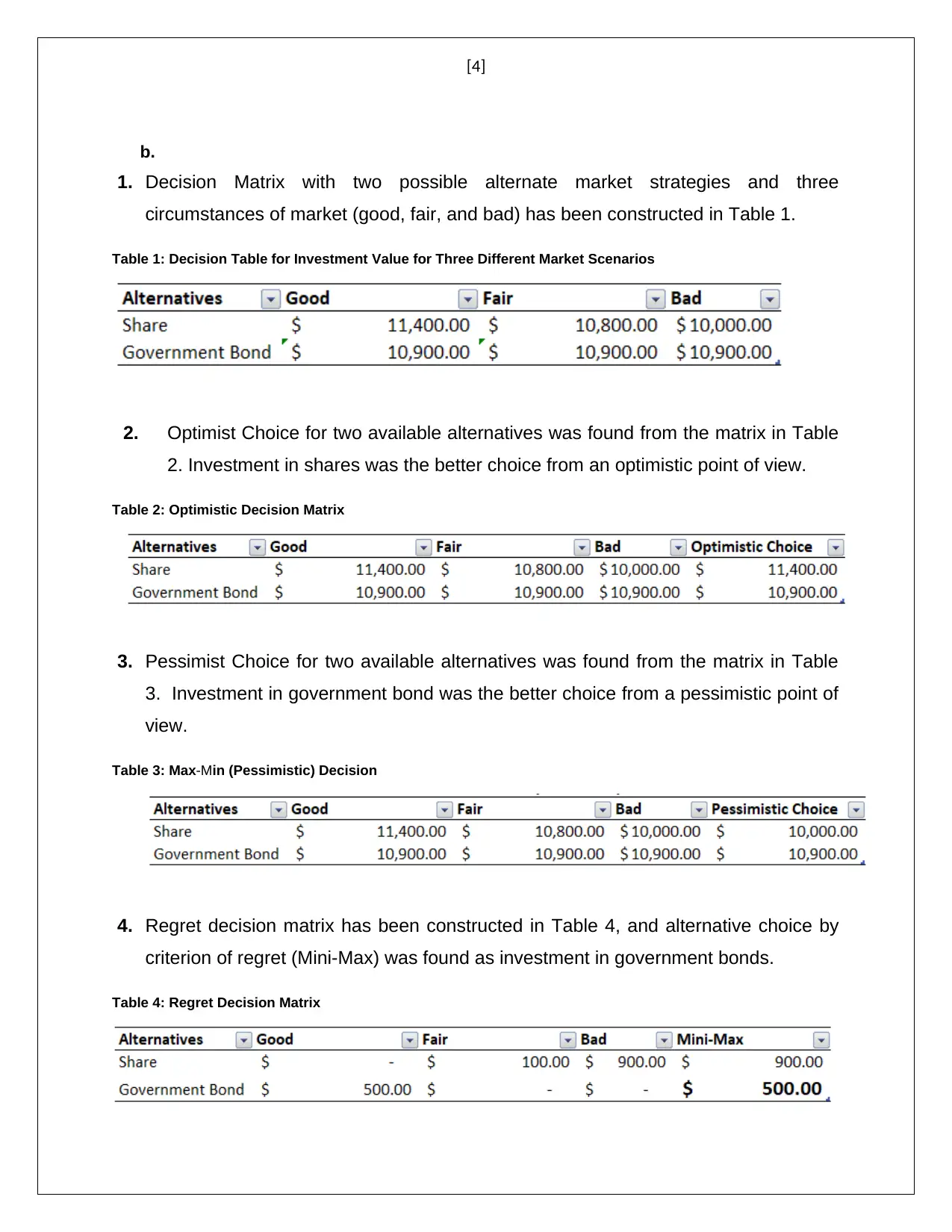
b.
1. Decision Matrix with two possible alternate market strategies and three
circumstances of market (good, fair, and bad) has been constructed in Table 1.
Table 1: Decision Table for Investment Value for Three Different Market Scenarios
2. Optimist Choice for two available alternatives was found from the matrix in Table
2. Investment in shares was the better choice from an optimistic point of view.
Table 2: Optimistic Decision Matrix
3. Pessimist Choice for two available alternatives was found from the matrix in Table
3. Investment in government bond was the better choice from a pessimistic point of
view.
Table 3: Max-Min (Pessimistic) Decision
4. Regret decision matrix has been constructed in Table 4, and alternative choice by
criterion of regret (Mini-Max) was found as investment in government bonds.
Table 4: Regret Decision Matrix
Paraphrase This Document
Need a fresh take? Get an instant paraphrase of this document with our AI Paraphraser
[5]
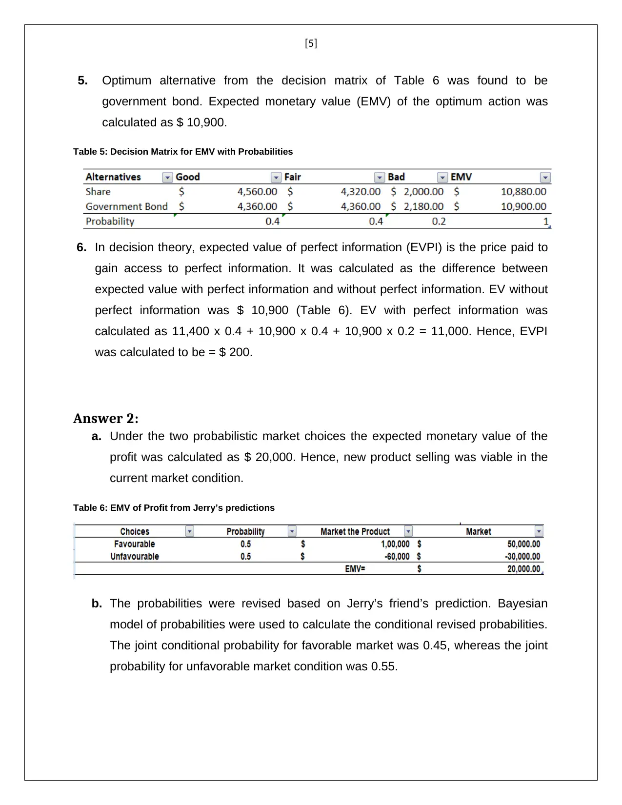
5. Optimum alternative from the decision matrix of Table 6 was found to be
government bond. Expected monetary value (EMV) of the optimum action was
calculated as $ 10,900.
Table 5: Decision Matrix for EMV with Probabilities
6. In decision theory, expected value of perfect information (EVPI) is the price paid to
gain access to perfect information. It was calculated as the difference between
expected value with perfect information and without perfect information. EV without
perfect information was $ 10,900 (Table 6). EV with perfect information was
calculated as 11,400 x 0.4 + 10,900 x 0.4 + 10,900 x 0.2 = 11,000. Hence, EVPI
was calculated to be = $ 200.
Answer 2:
a. Under the two probabilistic market choices the expected monetary value of the
profit was calculated as $ 20,000. Hence, new product selling was viable in the
current market condition.
Table 6: EMV of Profit from Jerry’s predictions
b. The probabilities were revised based on Jerry’s friend’s prediction. Bayesian
model of probabilities were used to calculate the conditional revised probabilities.
The joint conditional probability for favorable market was 0.45, whereas the joint
probability for unfavorable market condition was 0.55.
[6]
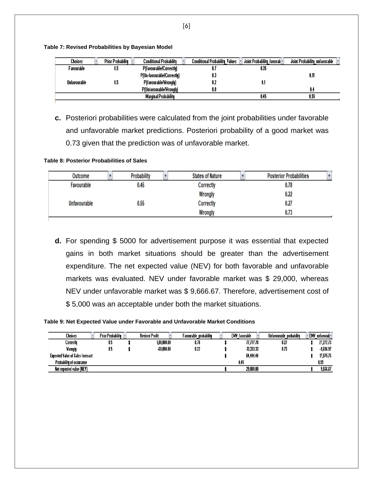
Table 7: Revised Probabilities by Bayesian Model
c. Posteriori probabilities were calculated from the joint probabilities under favorable
and unfavorable market predictions. Posteriori probability of a good market was
0.73 given that the prediction was of unfavorable market.
Table 8: Posterior Probabilities of Sales
d. For spending $ 5000 for advertisement purpose it was essential that expected
gains in both market situations should be greater than the advertisement
expenditure. The net expected value (NEV) for both favorable and unfavorable
markets was evaluated. NEV under favorable market was $ 29,000, whereas
NEV under unfavorable market was $ 9,666.67. Therefore, advertisement cost of
$ 5,000 was an acceptable under both the market situations.
Table 9: Net Expected Value under Favorable and Unfavorable Market Conditions
⊘ This is a preview!⊘
Do you want full access?
Subscribe today to unlock all pages.
Trusted by 1+ million students worldwide
[7]
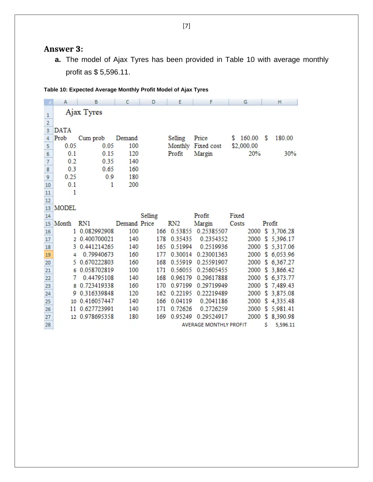
Answer 3:
a. The model of Ajax Tyres has been provided in Table 10 with average monthly
profit as $ 5,596.11.
Table 10: Expected Average Monthly Profit Model of Ajax Tyres
Answer 3:
a. The model of Ajax Tyres has been provided in Table 10 with average monthly
profit as $ 5,596.11.
Table 10: Expected Average Monthly Profit Model of Ajax Tyres
Paraphrase This Document
Need a fresh take? Get an instant paraphrase of this document with our AI Paraphraser
[8]
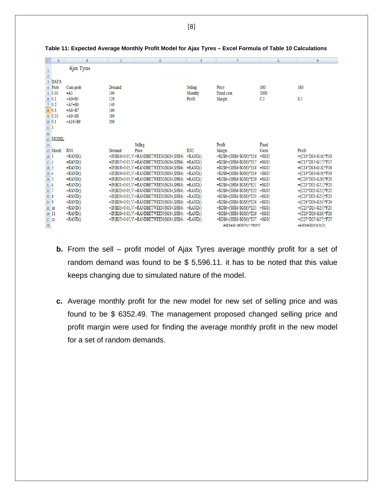
Table 11: Expected Average Monthly Profit Model for Ajax Tyres – Excel Formula of Table 10 Calculations
b. From the sell – profit model of Ajax Tyres average monthly profit for a set of
random demand was found to be $ 5,596.11. it has to be noted that this value
keeps changing due to simulated nature of the model.
c. Average monthly profit for the new model for new set of selling price and was
found to be $ 6352.49. The management proposed changed selling price and
profit margin were used for finding the average monthly profit in the new model
for a set of random demands.
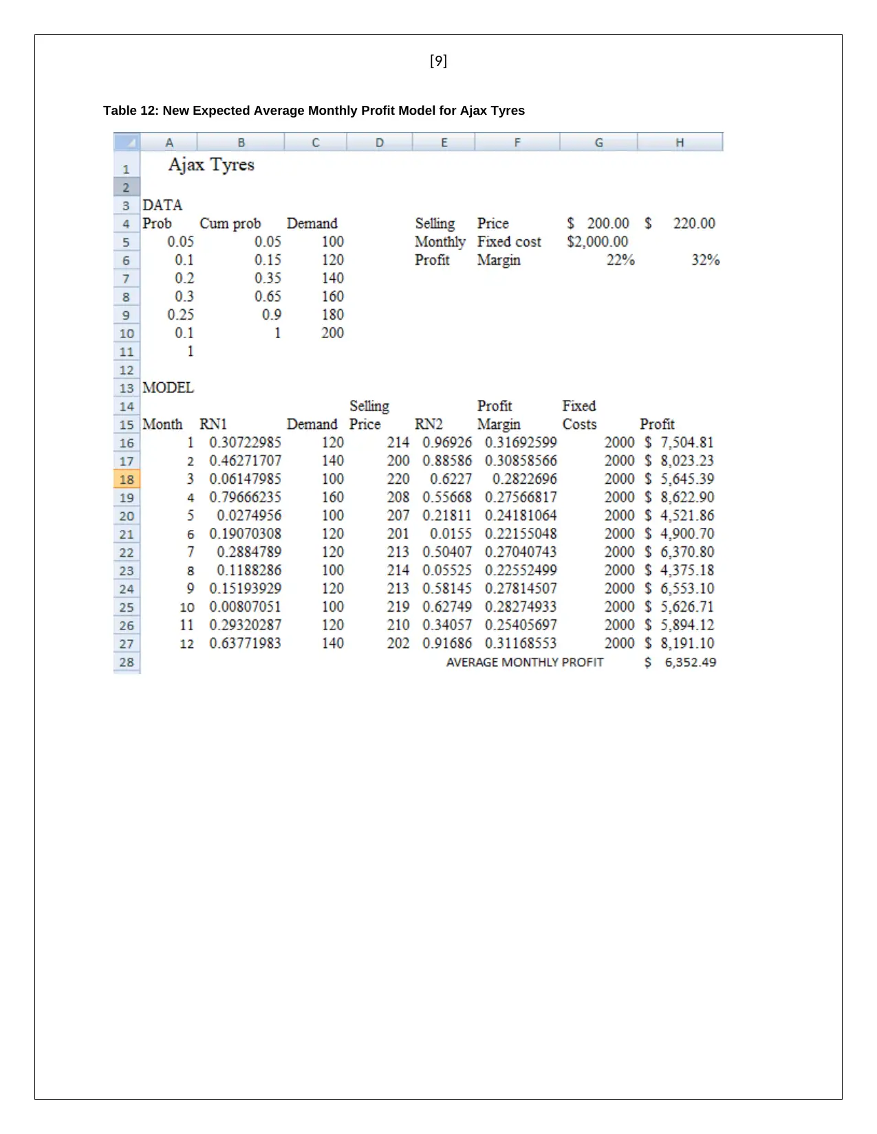
[9]
Table 12: New Expected Average Monthly Profit Model for Ajax Tyres
Table 12: New Expected Average Monthly Profit Model for Ajax Tyres
⊘ This is a preview!⊘
Do you want full access?
Subscribe today to unlock all pages.
Trusted by 1+ million students worldwide

[10]
To 18/ 09/ 2018
The Manager
Ajax Tyres
Subject: Summary of Yearly Profit of Ajax Tyres
Average monthly profit of Ajax Tyres from the sample analysis for 12 months was
found as $ 5,596.11. The simulated monthly demand model was quite efficient in
providing a comprehensible profit scenario. This efficient model was improvised
with new set of monthly average selling price per unit of tyre and new expected
range of profit margin. The average monthly simulated profit was $ 6352.49.
Hence, the new set of parameters was presumed to bring better profit figures.
For effective implementation of the new model market survey was essential,
especially for analysis of demand of tyres and price of different variants from
rivals. Increase in selling price might not increase margin of profit. The
assumptions behind the new model required to be verified with actual market
situations. For consistent market predictions, the simulated range of average
monthly profit would be reliable.
Thank you for the opportunity provided for analysing the sales of Ajax Tyres.
Regards
----------------------------
Paraphrase This Document
Need a fresh take? Get an instant paraphrase of this document with our AI Paraphraser
[11]
Answer 4:
a. The variable overhead cost per machine hour was calculated by high-low method.
The highest value of overhead cost was $ 80,000 and lowest value was $ 33,000.
The highest machine hour from the data was identified as 3800 and minimum
value was 1800. The variable cost was
OH Cost = ( highest cos t−lowest cos t )
Maximun MH−Minimum MH = ( 80000−33000 )
3800−1800 =23 .5
Hence, for 3,000 machine hours estimated variable OH cost was =23.5 x 3000 =
$ 70,500.
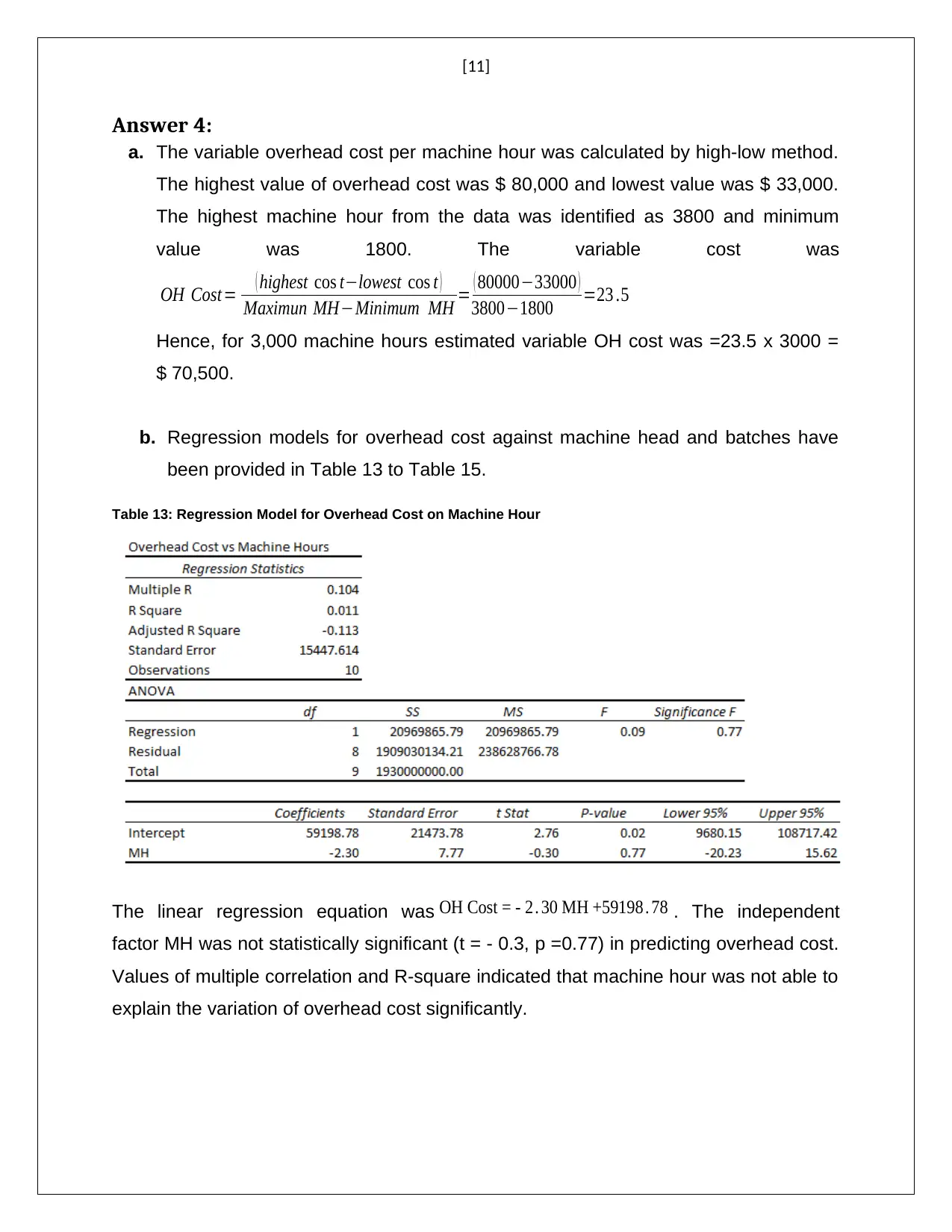
b. Regression models for overhead cost against machine head and batches have
been provided in Table 13 to Table 15.
Table 13: Regression Model for Overhead Cost on Machine Hour
The linear regression equation was OH Cost = - 2. 30 MH +59198 . 78 . The independent
factor MH was not statistically significant (t = - 0.3, p =0.77) in predicting overhead cost.
Values of multiple correlation and R-square indicated that machine hour was not able to
explain the variation of overhead cost significantly.
Answer 4:
a. The variable overhead cost per machine hour was calculated by high-low method.
The highest value of overhead cost was $ 80,000 and lowest value was $ 33,000.
The highest machine hour from the data was identified as 3800 and minimum
value was 1800. The variable cost was
OH Cost = ( highest cos t−lowest cos t )
Maximun MH−Minimum MH = ( 80000−33000 )
3800−1800 =23 .5
Hence, for 3,000 machine hours estimated variable OH cost was =23.5 x 3000 =
$ 70,500.
b. Regression models for overhead cost against machine head and batches have
been provided in Table 13 to Table 15.
Table 13: Regression Model for Overhead Cost on Machine Hour
The linear regression equation was OH Cost = - 2. 30 MH +59198 . 78 . The independent
factor MH was not statistically significant (t = - 0.3, p =0.77) in predicting overhead cost.
Values of multiple correlation and R-square indicated that machine hour was not able to
explain the variation of overhead cost significantly.
[12]
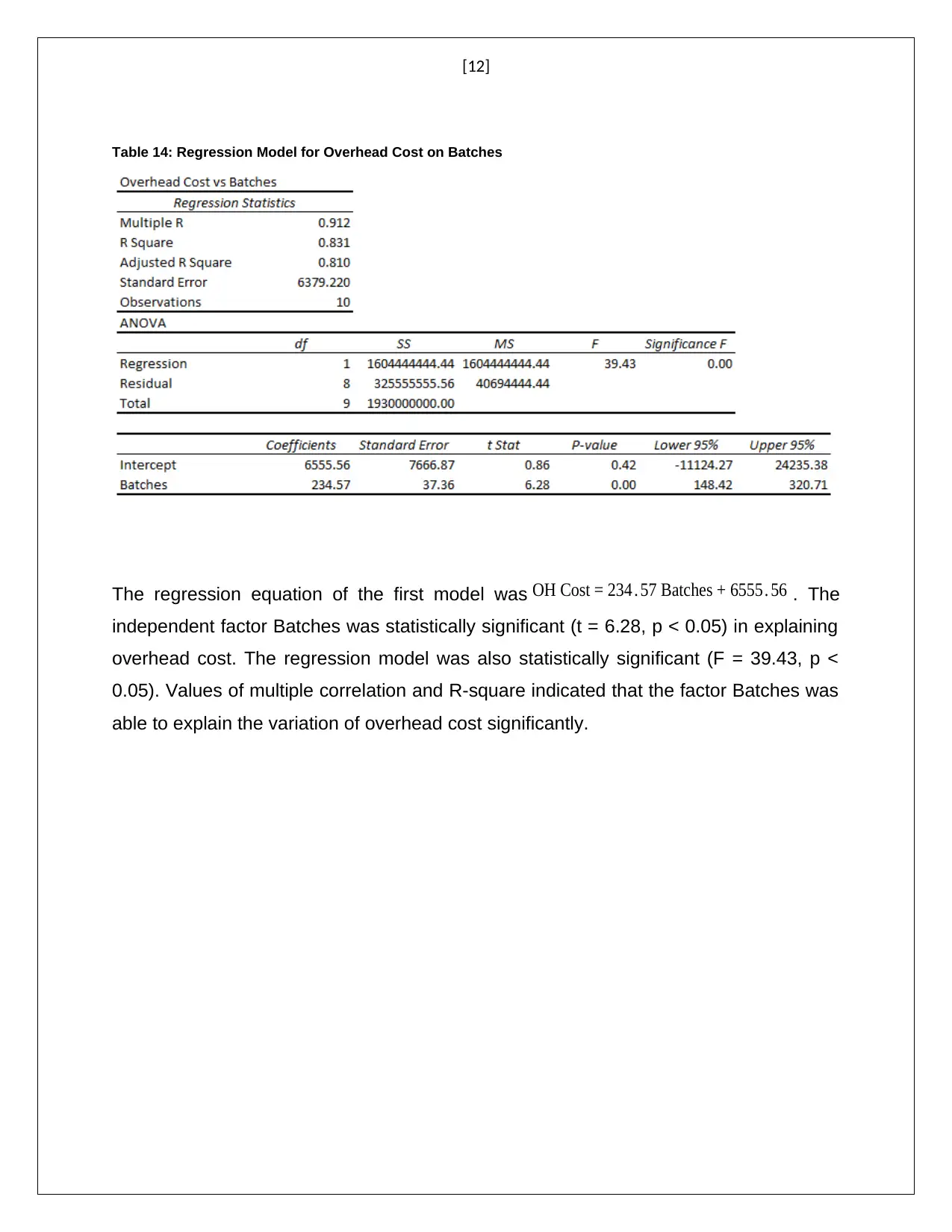
Table 14: Regression Model for Overhead Cost on Batches
The regression equation of the first model was OH Cost = 234 . 57 Batches + 6555. 56 . The
independent factor Batches was statistically significant (t = 6.28, p < 0.05) in explaining
overhead cost. The regression model was also statistically significant (F = 39.43, p <
0.05). Values of multiple correlation and R-square indicated that the factor Batches was
able to explain the variation of overhead cost significantly.
⊘ This is a preview!⊘
Do you want full access?
Subscribe today to unlock all pages.
Trusted by 1+ million students worldwide
1 out of 17
Related Documents


Your All-in-One AI-Powered Toolkit for Academic Success.
+13062052269
info@desklib.com
Available 24*7 on WhatsApp / Email
![[object Object]](/_next/static/media/star-bottom.7253800d.svg)
Unlock your academic potential
Copyright © 2020–2026 A2Z Services. All Rights Reserved. Developed and managed by ZUCOL.