Economics Homework: Demand Estimation, Elasticity and Market Share

This assignment analyzes the demand for a low-calorie, frozen microwavable food product. It begins by calculating various elasticities (price, income, cross, advertisement, and market) using a provided demand equation and discusses their implications for short-term and long-term pricing strategies. ...Read More

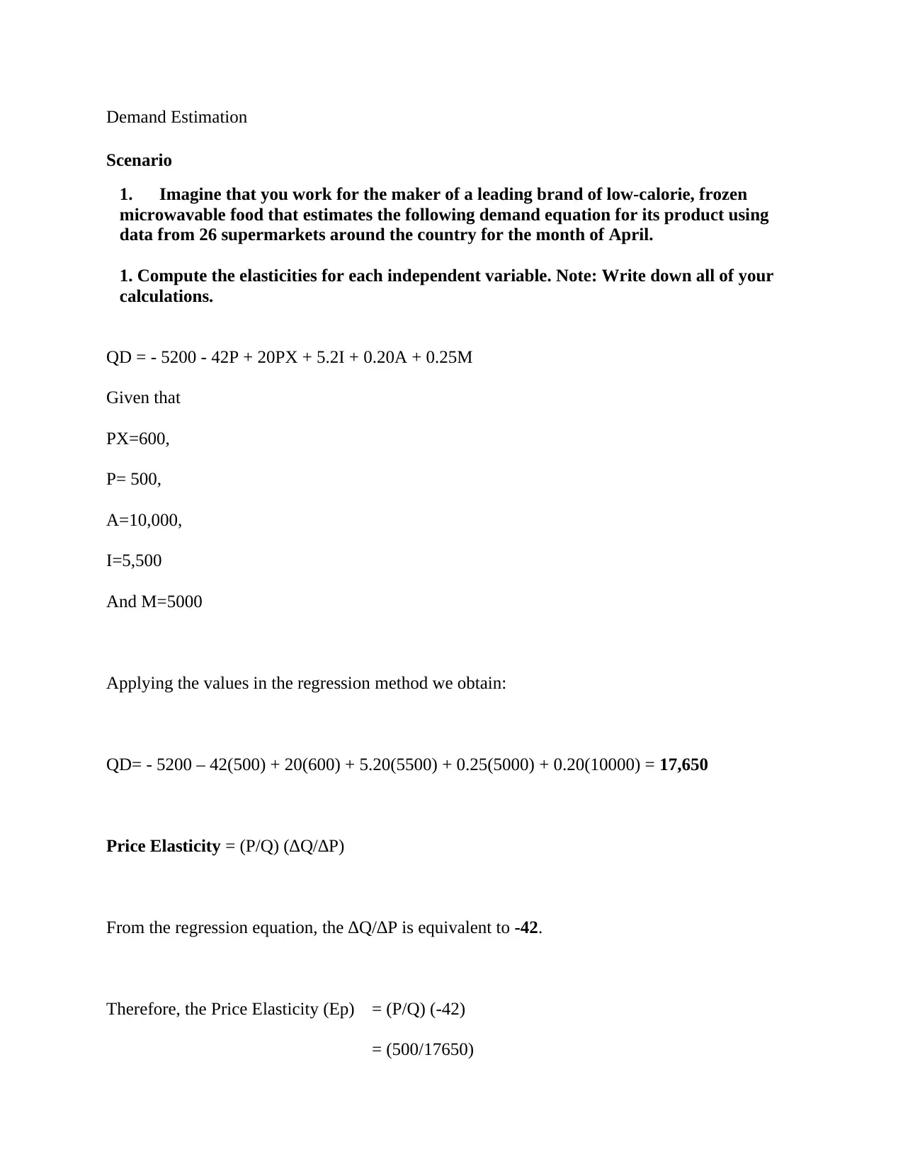
Demand Estimation
Scenario
1. Imagine that you work for the maker of a leading brand of low-calorie, frozen
microwavable food that estimates the following demand equation for its product using
data from 26 supermarkets around the country for the month of April.
1. Compute the elasticities for each independent variable. Note: Write down all of your
calculations.
QD = - 5200 - 42P + 20PX + 5.2I + 0.20A + 0.25M
Given that
PX=600,
P= 500,
A=10,000,
I=5,500
And M=5000
Applying the values in the regression method we obtain:
QD= - 5200 – 42(500) + 20(600) + 5.20(5500) + 0.25(5000) + 0.20(10000) = 17,650
Price Elasticity = (P/Q) (∆Q/∆P)
From the regression equation, the ∆Q/∆P is equivalent to -42.
Therefore, the Price Elasticity (Ep) = (P/Q) (-42)
= (500/17650)

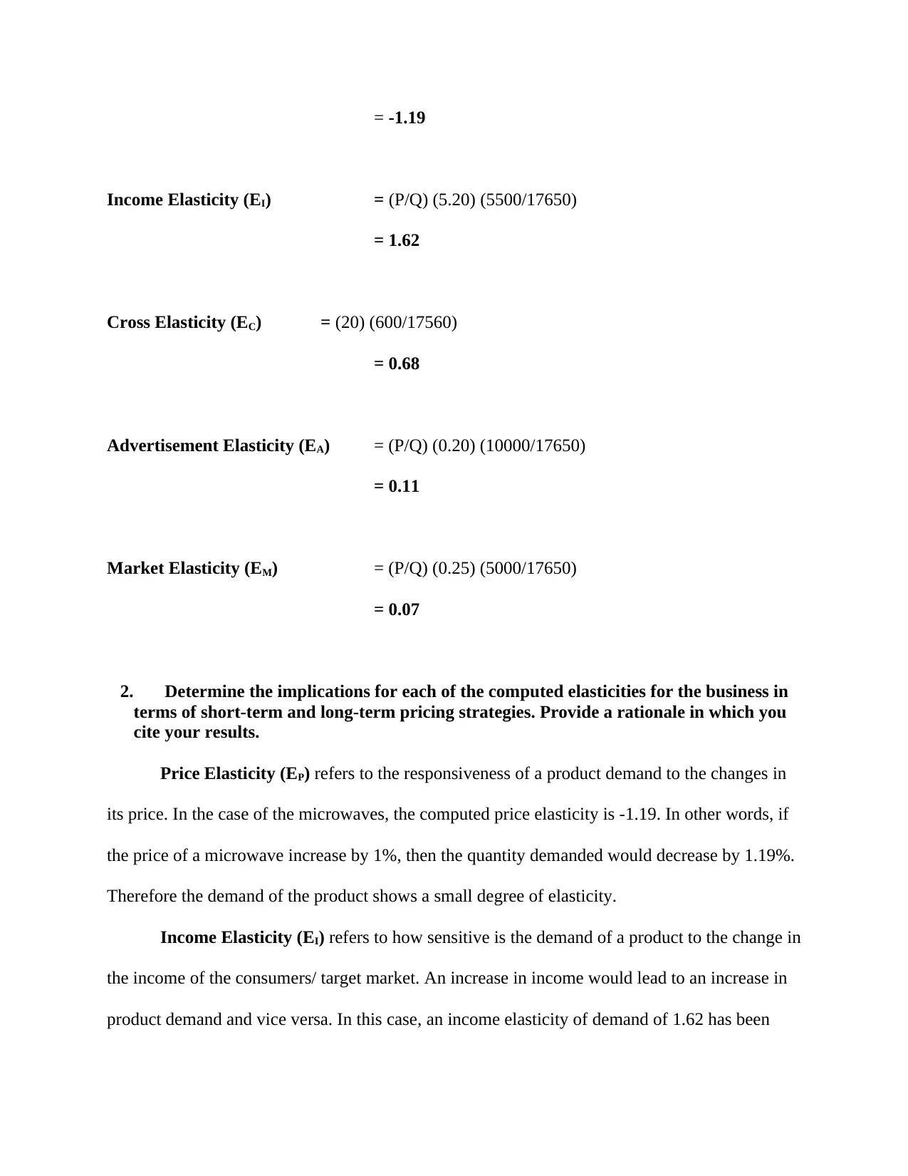
= -1.19
Income Elasticity (EI) = (P/Q) (5.20) (5500/17650)
= 1.62
Cross Elasticity (EC) = (20) (600/17560)
= 0.68
Advertisement Elasticity (EA) = (P/Q) (0.20) (10000/17650)
= 0.11
Market Elasticity (EM) = (P/Q) (0.25) (5000/17650)
= 0.07
2. Determine the implications for each of the computed elasticities for the business in
terms of short-term and long-term pricing strategies. Provide a rationale in which you
cite your results.
Price Elasticity (EP) refers to the responsiveness of a product demand to the changes in
its price. In the case of the microwaves, the computed price elasticity is -1.19. In other words, if
the price of a microwave increase by 1%, then the quantity demanded would decrease by 1.19%.
Therefore the demand of the product shows a small degree of elasticity.
Income Elasticity (EI) refers to how sensitive is the demand of a product to the change in
the income of the consumers/ target market. An increase in income would lead to an increase in
product demand and vice versa. In this case, an income elasticity of demand of 1.62 has been

computed. This shows that if the average income increases by 1%, then the product demand
would subsequently increase 1.62%. The microwave product shows elasticity. This nature of
elasticity depicts that the company can choose to increase the product price when there is an
average increase of income (Bishop, Parrott , Martie , & Miller, 2014).
Cross Elasticity (EC) refers to the level of responsiveness is the demand of a product
influenced by the change in the price of a competitor’s product. The computed cross-price
elasticity of demand is 0.68. The figure implies that if the price of a similar product by
competitors increase by 1% then the quantity demanded of the microwave would increase with
0.68%. This can be explained as a fairly inelastic product in relation to the competitor’s price
(Raisová & Ďurčová, 2014).
Advertisement Elasticity (EA) refers to how sensitive is the demand of the product to the
changes of the advertising/ promotional expenses. In other words, how do the changes in the
promotional expenses influence the demand for the commodity? In this case, the advertisement
elasticity of demand was computed as 0.11. The results show that an increase of advertising
expenses by 1% would lead to an increase in demand for the product by 0.11%. This shows that
advertisement has an inelastic relationship with the product demand. An increase in the amount
invested in the advertisement should not automatically lead to an increased price of the product
(Gillespie, 2014). The firm should not find an excuse in the increase advertisement expenses to
increase the price of the product because the consumers are likely to switch to the competitor’s
product.
Market Elasticity (EM) refers to how responsive is the demand of the precut to the
changes in the market. Market elasticity evaluates how elastic is the demand of the product to the
external forces which influence the market. The Microwave ovens have a market elasticity of

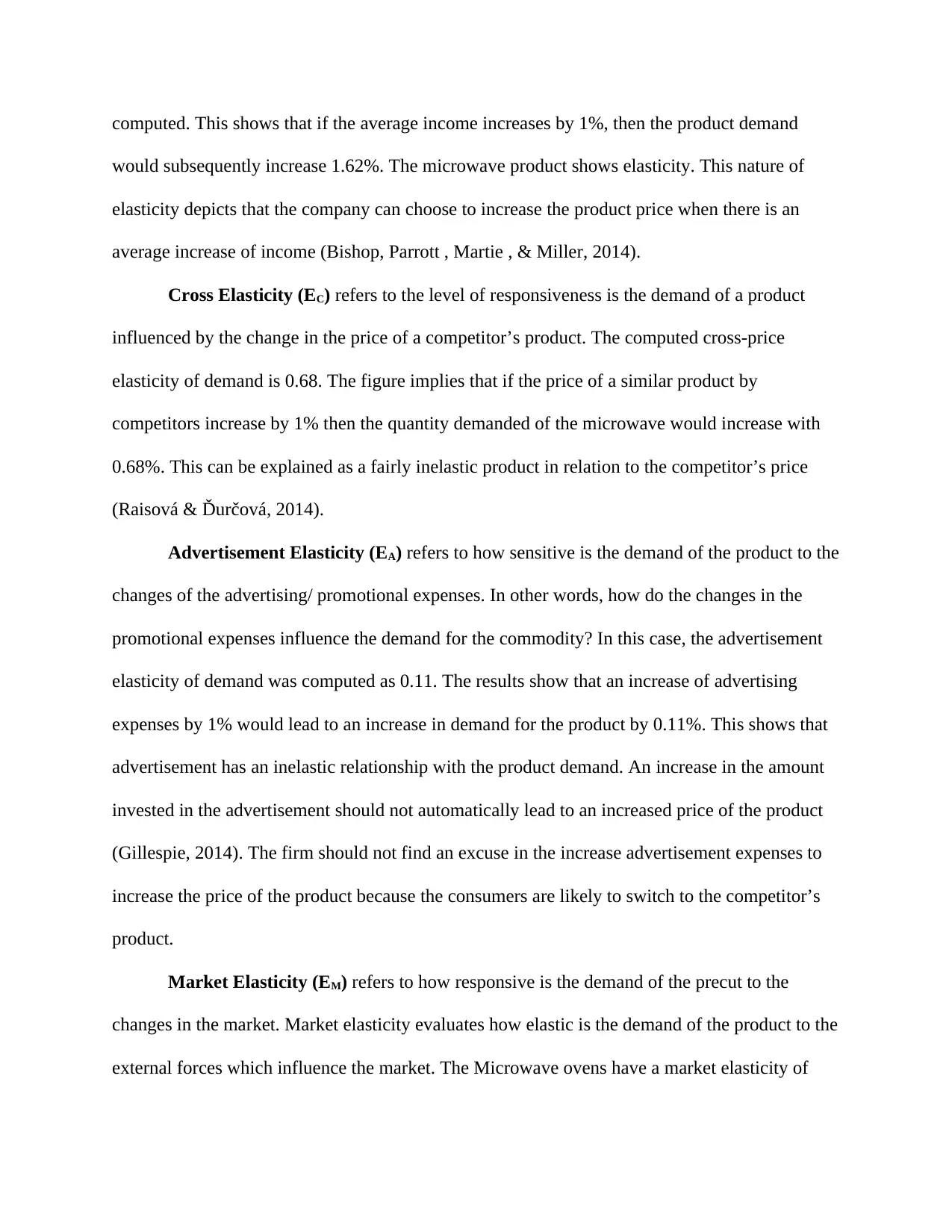
demand of 0.07. The result shows that the demand of ovens would increase by 0.07% when the
number of the oven in the market increases by 1%. The EM shows an inelastic demand; the
number of ovens in the market cannot be relied upon as a factor to impact the quantity demand
(Kash, 2002).
3. Recommend whether you believe that this firm should or should not cut its price to
increase its market share. Provide support for your recommendation.
According to the law of demand, the lower the price of a commodity, the higher the
quantity demanded. The computed price elasticity was -1.19 which shows that the increase in
price would lead to the reduction of quantity demanded. Subsequently, if the price is decreased
by 1% the quantity demanded would increase by 1.1.9%. Further reduction of the price would
increase the number of sales and hence an increase in the market share. Therefore, to gain a
larger market share, the company should reduce the price of its microwave ovens (Marshall,
2008).
4. Assume that all the factors affecting demand in this model remain the same, but
that the price has changed. Further assume that the price changes are 100, 200, 300,
400, 500, 600 cents.
Using the regression equation QD = - 5200 - 42P + 20PX + 5.2I + 0.20A + 0.25M, the
quantity demanded are;
QD = - 5200 - 42P + 20PX + 5.2I + 0.20A + 0.25M
= - 5200-42P +20(600) + 5.20(5500) + 0.25(5000) + 0.20(10000)
QD = 38650-42P
When
P= 100, QD= 34,450

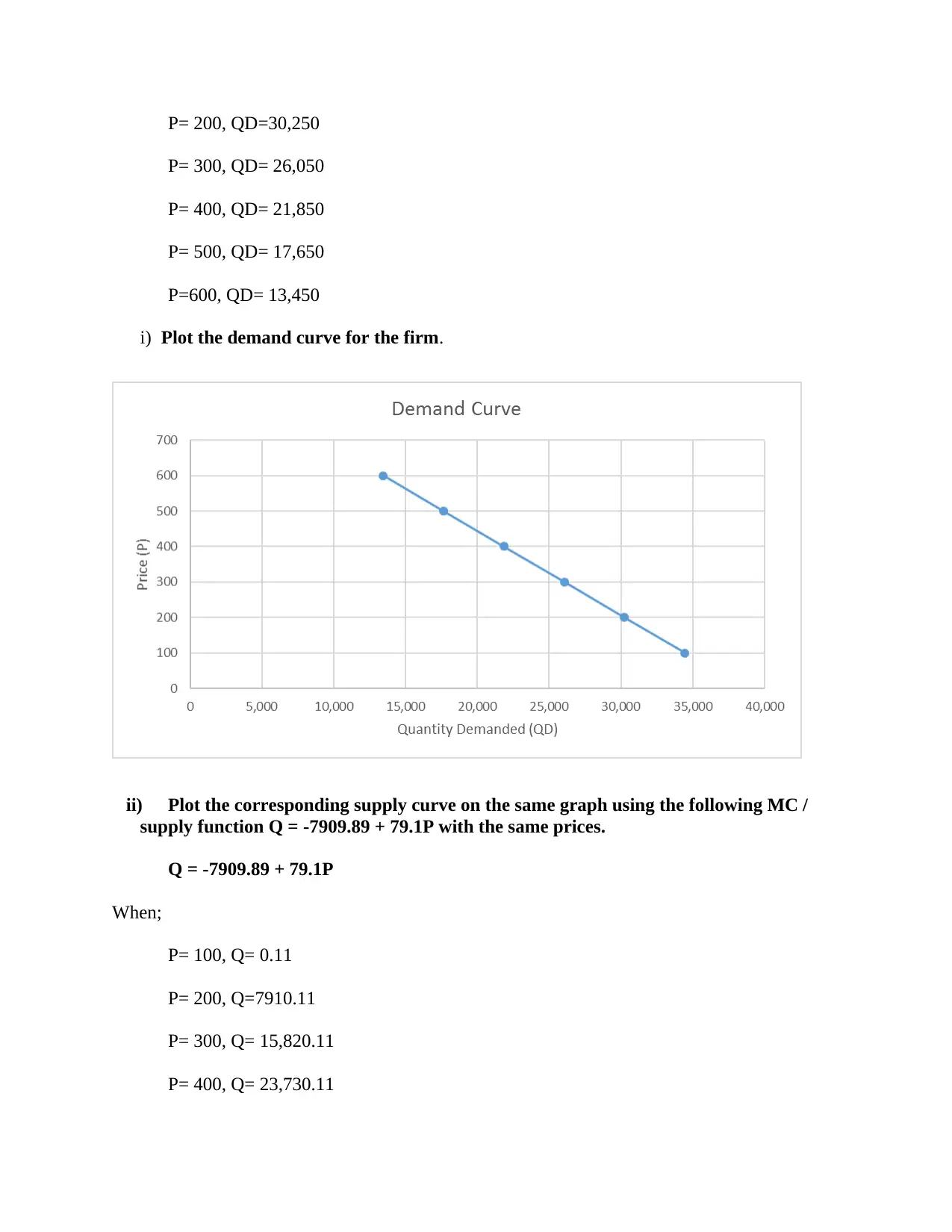
P= 200, QD=30,250
P= 300, QD= 26,050
P= 400, QD= 21,850
P= 500, QD= 17,650
P=600, QD= 13,450
i) Plot the demand curve for the firm.
ii) Plot the corresponding supply curve on the same graph using the following MC /
supply function Q = -7909.89 + 79.1P with the same prices.
Q = -7909.89 + 79.1P
When;
P= 100, Q= 0.11
P= 200, Q=7910.11
P= 300, Q= 15,820.11
P= 400, Q= 23,730.11

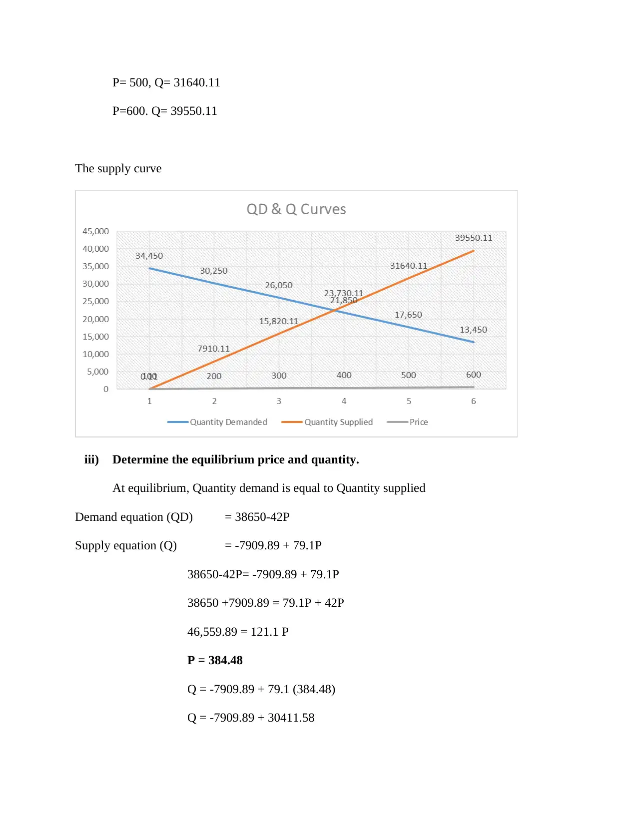
P= 500, Q= 31640.11
P=600. Q= 39550.11
The supply curve
iii) Determine the equilibrium price and quantity.
At equilibrium, Quantity demand is equal to Quantity supplied
Demand equation (QD) = 38650-42P
Supply equation (Q) = -7909.89 + 79.1P
38650-42P= -7909.89 + 79.1P
38650 +7909.89 = 79.1P + 42P
46,559.89 = 121.1 P
P = 384.48
Q = -7909.89 + 79.1 (384.48)
Q = -7909.89 + 30411.58

Q = 22,501.69
iv) Outline the significant factors that could cause changes in supply and demand for
the low-calorie, frozen microwavable food. Determine the primary manner in which
both the short-term and the long-term changes in market conditions could impact the
demand for, and the supply, of the product.
The equilibrium price and quantity occur at the point of interception between the supply
and demand curves. The equilibrium price and quantity for the microwave oven are 384.84 and
22,501.69 respectively.
Changes in the demand curve are caused by several factors such as changes in the
consumers’ income, change in the price of the substitute products, pricing of correlated products
and the change of the consumers’ taste and preferences. In the other hand, changes in the supply
curve are influenced by technological advancement, availability of labour and raw material and
number of products supplied (Gillespie, 2014).
v) Indicate the crucial factors that could cause rightward shifts and leftward shifts of
the demand and supply curves for the low-calorie, frozen microwavable food.
The rightward shift is as a result of an increase in the quantity demanded. There are
several factors that lead to the shift of the demand curve to the right. Example of these factors
are; a) Increase of the consumers’ income; b) increase of the consumers’ taste and preferences; c)
expected a future increase of the product price; and d) government influences (Marshall, 2008).
The leftward shift is as a result of a decrease in the quantity demanded. There are several factors
that lead to the shift of the demand curve to the left. Example of these factors are; a) expected a
future decrease of the product price; b) decrease of the consumers’ taste and preferences; c)
decrease of the consumers’ income; and d) ) government influences (Raisová & Ďurčová, 2014).

Availability of raw materials, government subsidies, and technological improvements
leading to a shift of the supply curve to the right. Likewise, mechanization, as a result of
technological improvement results to increased production prompting the shift of the supply
curve to the right.
The increase of labour price, decrease or raw material and labour available and increase
in taxes causes the supply curve to shift to the left. All these factors lead to a reduction in
production leading to the leftward shift (Gillespie, 2014).

References
Bishop, S., Parrott , C., Martie , C., & Miller, R. (2014). Kaplan AP
Macroeconomics/Microeconomics. New Delhi: Kaplan Publishing.
Gillespie, A. (2014). Foundations of Economics. New Jersey: Oxford University Press.
Kash, R. (2002). The New Law of Demand and Supply: The Revolutionary New Demand
Strategy for Faster Growth and Higher Profits. New York: Doubleday Business.
Marshall, A. (2008). Principles of Economics. London, UK: Macmillan and Company.
Raisová, M., & Ďurčová, J. (2014). Economic Growth-supply and Demand Perspectiv. Procedia
Economics and Finance, Volume 15, Pages 184-191.