Microeconomics Analysis: Demand, Supply, and Costs of Production

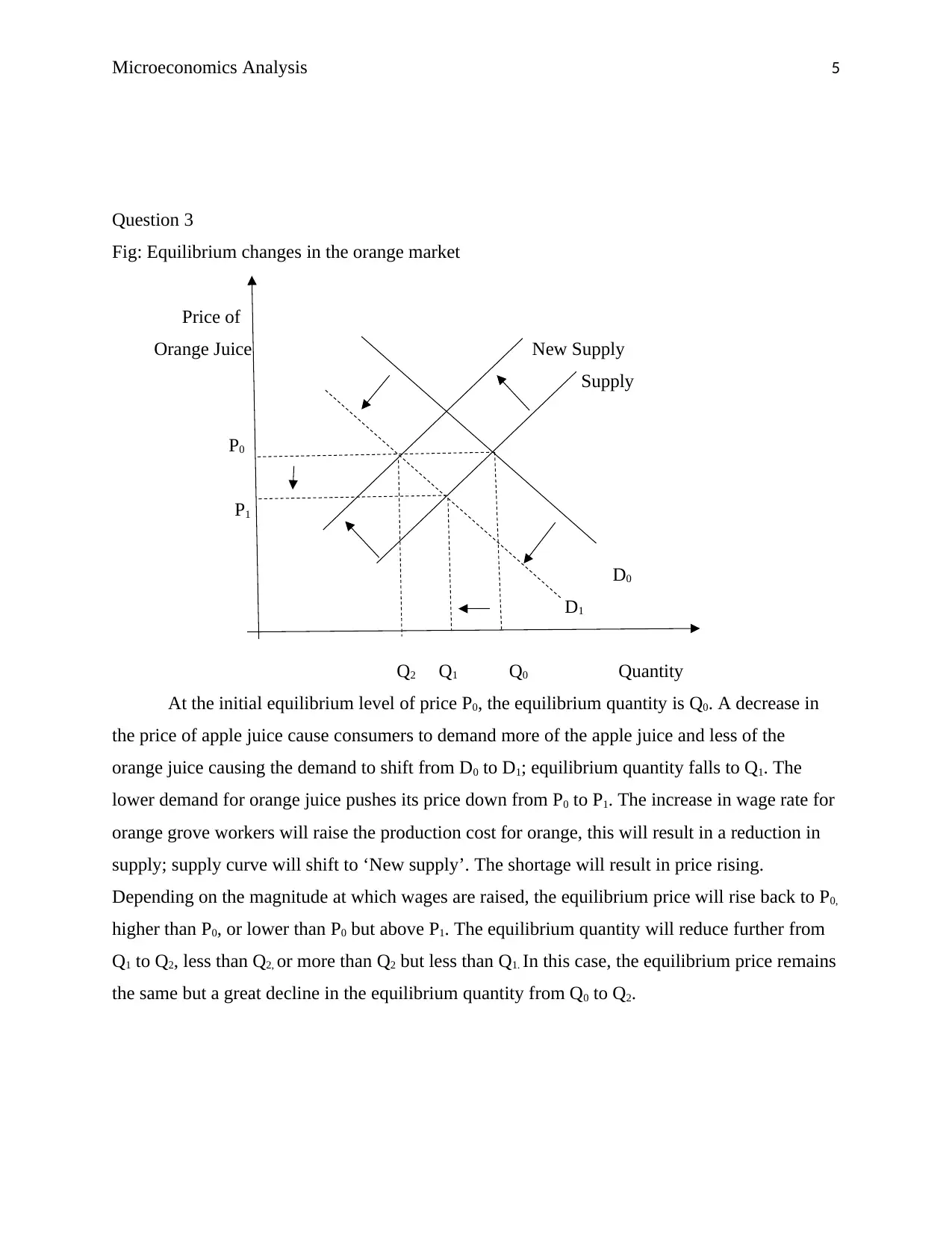
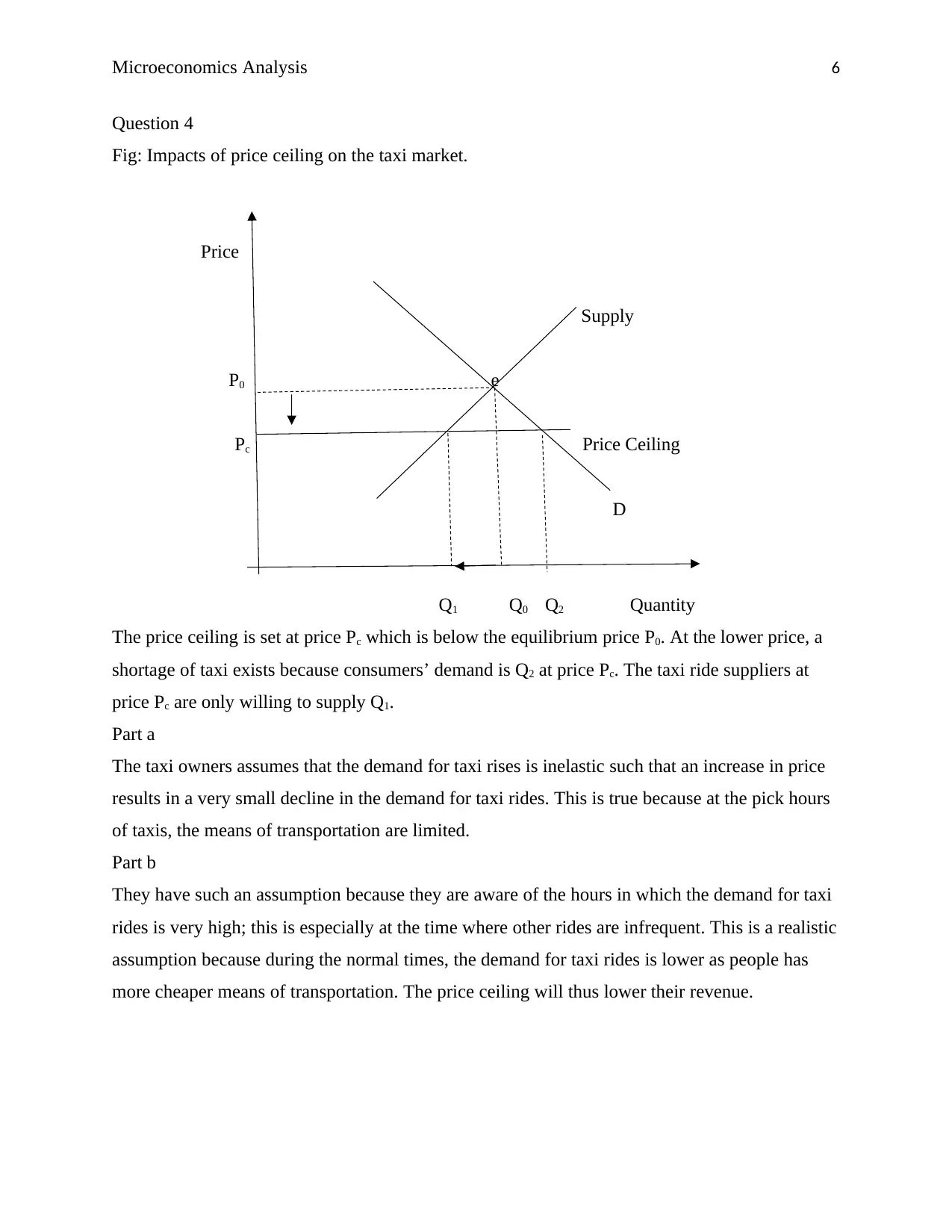
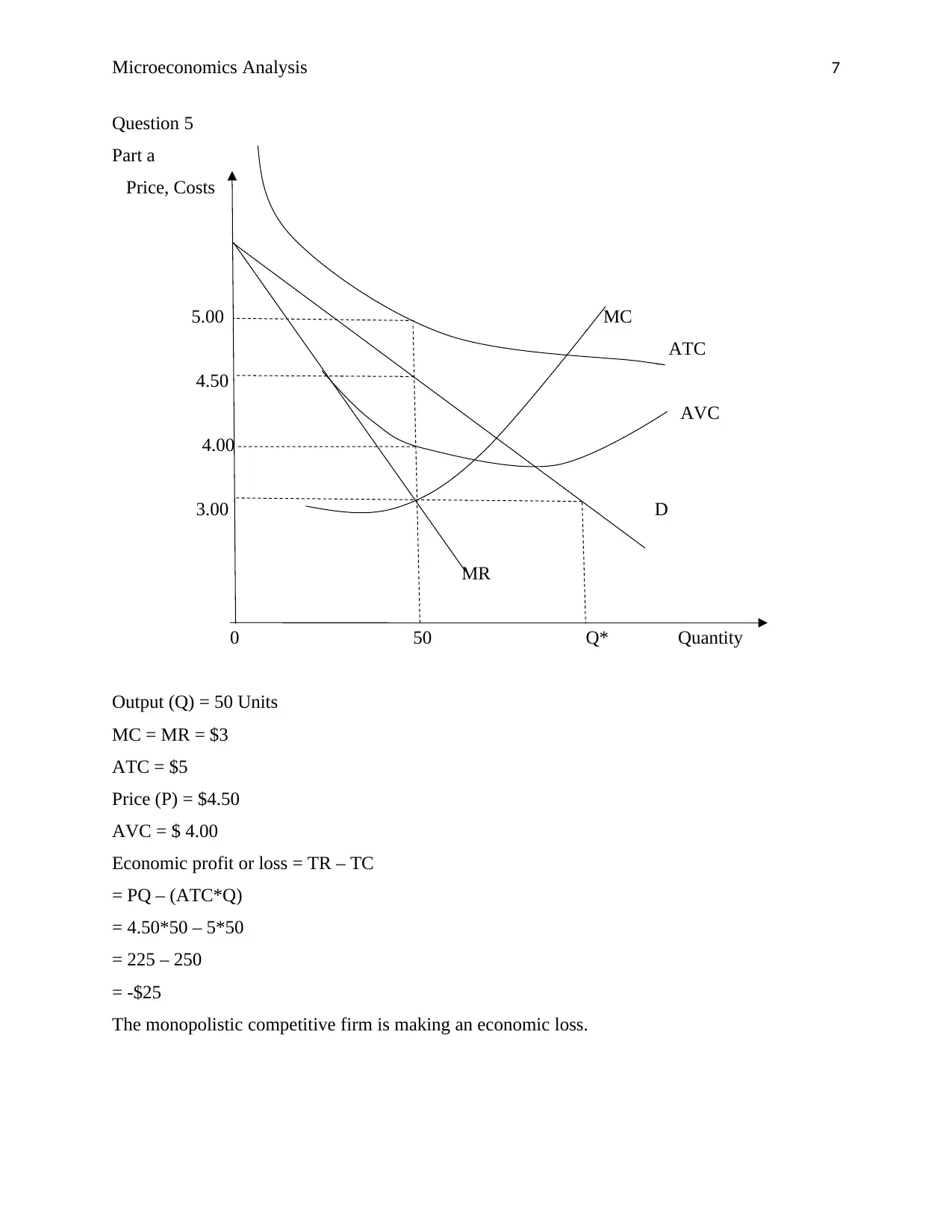
This report provides a comprehensive microeconomic analysis of demand, supply, and production costs. It addresses key concepts such as demand and supply curves, market equilibrium, and the impact of various factors on these dynamics. The report examines scenarios including shifts in demand due to non-price factors, the effects of poor harvests on market supply and prices, and the consequences of price ceilings. It also delves into the cost structures of firms operating in monopolistically competitive markets, analyzing profit or loss situations and output recommendations. The analysis uses graphs to illustrate these economic principles, offering a visual representation of market changes and equilibrium shifts. The report concludes with a discussion of the factors influencing demand elasticity and the strategic decisions of firms in response to market conditions.

Running Head: Microeconomics Analysis
Demand and Supply and the Costs of Production
Student Name
Institutional Affiliation
Course/Number
Instructor Name
Due Date

Microeconomics Analysis 2
Demand and Supply and the Costs of Production
Question 1
No, the demand curve always slopes downwards, the far it can go as far as price and other factors
are concerned is to be horizontal but it cannot slope upwards; a horizontal demand curve means
that it’s perfectly inelastic. The upward sloping curve is the supply curve; the supply curve could
even be vertical when it’s perfectly inelastic.
Fig: Slope and shifting of the demand curve
Supply
P1
P0
D1
D0
Q0 Q1
At equilibrium, Q0 quantity of beef are demanded at price P0. In the normal cases, a price
increment results in demand falling. However, price can rise and the demand still goes up. How
will this happen? If price rises from P0 to p1, demand is expected to fall, however a non-price
factor pushes the demand for beef causing a rightward shift of the demand curve from D0 to D1
(Amadeo, 2018). One of the factor responsible for this could be for instance an increase in the
price for chicken meat a substitute for beef. This will lower chicken demand and raise beef
demand.

Microeconomics Analysis 3
Question 2
Part a
Fig: Impacts of poor wine-grains harvest on the French Wine market
New Supply
Supply
P1
P0
D
Qd Q0 Qs
The poor harvest will cause a shortage shown in the above graph since the supply curve will shift
to ‘New supply curve’; this is a shift from supplying Q0 to supplying Qd (Ctvnews.ca, 2017). A
shortage push the price for French wines upwards (Kottasová, 2017).

Microeconomics Analysis 4
Part b
Fig: Impacts of highly priced French wine on Australian wine Market.
Price of
Australian
Wine Supply
P1
P0
D1
D0
Q0 Q1 Quantity
Initially, the equilibrium Australian demand for wine is Q0 and price is P0. After the French wine
goes up owing to the shortage, the Australian producers export more wine to take advantage of
this market niche. Given the demand in France and the existing demand in Australia, the two
markets creates a higher demand for Australian wine. The increased demand causes price for
wine in Australia to also go up.

Microeconomics Analysis 5
Question 3
Fig: Equilibrium changes in the orange market
Price of
Orange Juice New Supply
Supply
P0
P1
D0
D1
Q2 Q1 Q0 Quantity
At the initial equilibrium level of price P0, the equilibrium quantity is Q0. A decrease in
the price of apple juice cause consumers to demand more of the apple juice and less of the
orange juice causing the demand to shift from D0 to D1; equilibrium quantity falls to Q1. The
lower demand for orange juice pushes its price down from P0 to P1. The increase in wage rate for
orange grove workers will raise the production cost for orange, this will result in a reduction in
supply; supply curve will shift to ‘New supply’. The shortage will result in price rising.
Depending on the magnitude at which wages are raised, the equilibrium price will rise back to P0,
higher than P0, or lower than P0 but above P1. The equilibrium quantity will reduce further from
Q1 to Q2, less than Q2, or more than Q2 but less than Q1. In this case, the equilibrium price remains
the same but a great decline in the equilibrium quantity from Q0 to Q2.

Microeconomics Analysis 6
Question 4
Fig: Impacts of price ceiling on the taxi market.
Price
Supply
P0 e
Pc Price Ceiling
D
Q1 Q0 Q2 Quantity
The price ceiling is set at price Pc which is below the equilibrium price P0. At the lower price, a
shortage of taxi exists because consumers’ demand is Q2 at price Pc. The taxi ride suppliers at
price Pc are only willing to supply Q1.
Part a
The taxi owners assumes that the demand for taxi rises is inelastic such that an increase in price
results in a very small decline in the demand for taxi rides. This is true because at the pick hours
of taxis, the means of transportation are limited.
Part b
They have such an assumption because they are aware of the hours in which the demand for taxi
rides is very high; this is especially at the time where other rides are infrequent. This is a realistic
assumption because during the normal times, the demand for taxi rides is lower as people has
more cheaper means of transportation. The price ceiling will thus lower their revenue.

Microeconomics Analysis 7
Question 5
Part a
Price, Costs
5.00 MC
ATC
4.50
AVC
4.00
3.00 D
MR
0 50 Q* Quantity
Output (Q) = 50 Units
MC = MR = $3
ATC = $5
Price (P) = $4.50
AVC = $ 4.00
Economic profit or loss = TR – TC
= PQ – (ATC*Q)
= 4.50*50 – 5*50
= 225 – 250
= -$25
The monopolistic competitive firm is making an economic loss.

Microeconomics Analysis 8
Part b
The output recommendation for this firm is level Q* in the diagram above since it’s the
competitive quantity.

Microeconomics Analysis 9
Bibliography
Amadeo, K. (2018). When Demand Changes No Matter the Price. Retrieved from
https://www.thebalance.com/shift-in-demand-curve-when-price-doesn-t-matter-3305720
Ctvnews.ca. (2017). Poor grape harvest leads to record low French wine production. Retrieved
from https://www.ctvnews.ca/lifestyle/poor-grape-harvest-leads-to-record-low-french-
wine-production-1.3514773.
Evans, S. (2017). Poor French grape harvest a dilemma for Treasury Wine Estates. Retrieved
from http://www.afr.com/business/agriculture/poor-french-grape-harvest-a-dilemma-for-
treasury-wine-estates-20170906-gyc7zp.
Kottasová, I. (2017). Disastrous harvest means wine prices could be going up. Retrieved from
http://money.cnn.com/2017/10/13/news/wine-shortage-europe-weather-california-fire/
index.html.
Reff, S. (2015). Monopolistic Competition. Retrieved from
http://reffonomics.com/MonopolisticCompetition.html.
Woodruff, J. (2018). What Are the Four Factors That Cause a Shift in Demand? Retrieved from
http://smallbusiness.chron.com/four-factors-cause-shift-demand-56212.html.