BUSM20000D Research Project: Demographic Data Analysis Report

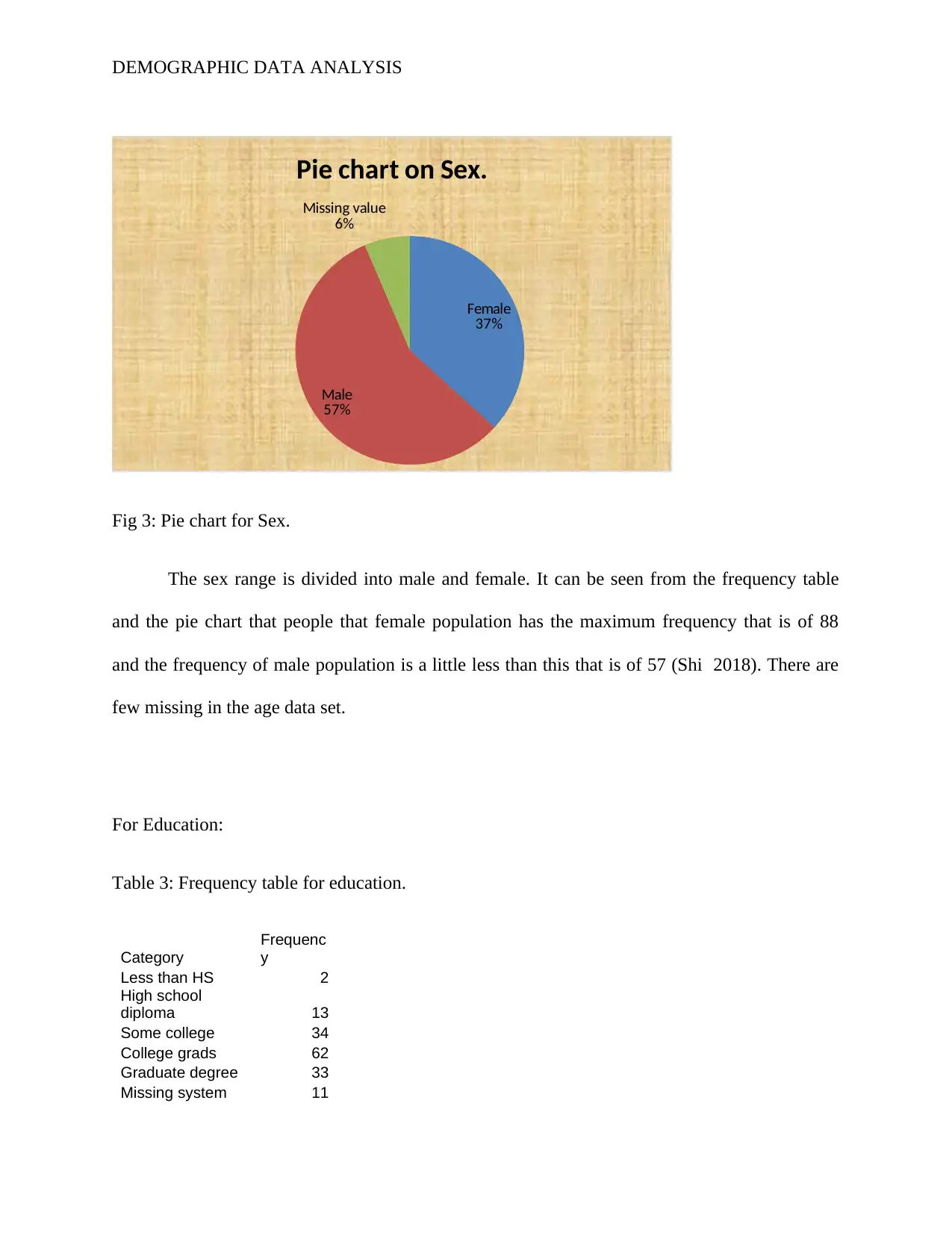
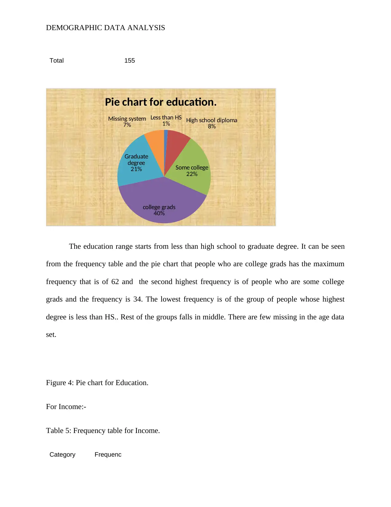
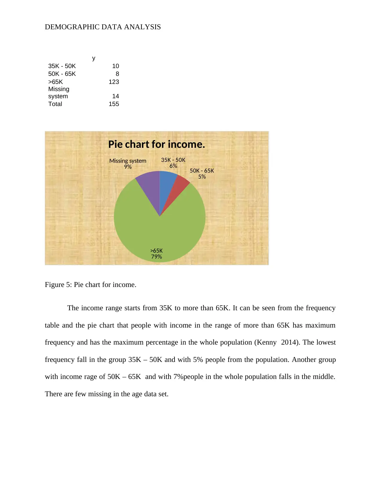
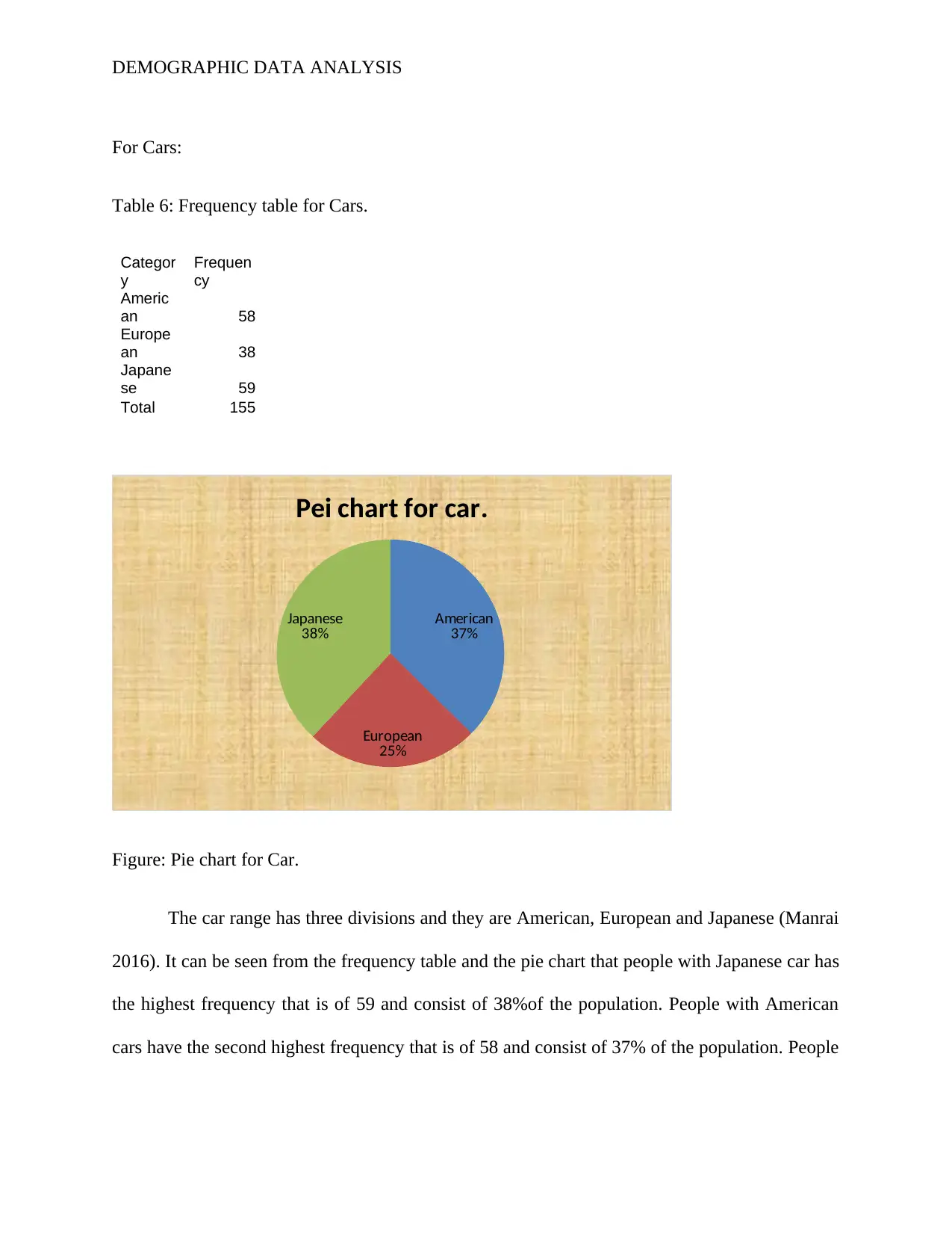
This report presents a demographic data analysis, examining the distribution of variables such as age, sex, education, income, and car ownership within a sample. Descriptive statistics, including frequency tables and pie charts, are used to illustrate the data. The report further explores relationships between categorical variables using cross-tabulations and chi-square tests, as well as t-tests and ANOVA to assess differences between groups. The analysis includes hypothesis testing related to sex and education, car ownership and sense of accomplishment, age and sex, and sex and education, providing insights into the statistical significance of observed associations. Desklib provides access to this and similar documents, enhancing students' understanding of statistical analysis.

0Running head: DEMOGRAPHIC DATA ANALYSIS
DEMOGRAPHIC DATA ANALYSIS
Name of the student
Name of the university
Author’s note

DEMOGRAPHIC DATA ANALYSIS
Executive summary

DEMOGRAPHIC DATA ANALYSIS
Table of Contents
Introduction......................................................................................................................................2
Analysis...........................................................................................................................................2
Conclusion.......................................................................................................................................2
References........................................................................................................................................3
Appendix..........................................................................................................................................4

DEMOGRAPHIC DATA ANALYSIS
Introduction
Analysis
Descriptive statistics of demographic variable of the sample:
For age:
Table 1: Frequency table for Age
Categorie
s
Frequenc
y
Others 1
35 or less 20
36-45 45
46-55 51
56-65 18
65+ 10
Missing
data 10
Total 145
Others
1% 35 or less
13%
36-45
29%
46-55
33%
56-65
12%
65+
6%
Missing data
6%
Pie chart on age.

DEMOGRAPHIC DATA ANALYSIS
Fig 1: Pie chart for Age.
The age range starts from 0 years to more than 65 years. It can be seen from the
frequency table and the pie chart that people with ages in the range of 46 – 55 has the maximum
frequency that is of 51 the second highest frequency is of people in the age range 36 – 45. The
lowest frequency is of the group with age 65+ (Sharpe 2015). Rest of the groups of ages falls in
middle. There are few missing in the age data set.
For Sex:
Table 2: Frequency table for Sex
Categories
Frequenc
y
Female 57
Male 88
Missing
value 10
Total 155

DEMOGRAPHIC DATA ANALYSIS
Female
37%
Male
57%
Missing value
6%
Pie chart on Sex.
Fig 3: Pie chart for Sex.
The sex range is divided into male and female. It can be seen from the frequency table
and the pie chart that people that female population has the maximum frequency that is of 88
and the frequency of male population is a little less than this that is of 57 (Shi 2018). There are
few missing in the age data set.
For Education:
Table 3: Frequency table for education.
Category
Frequenc
y
Less than HS 2
High school
diploma 13
Some college 34
College grads 62
Graduate degree 33
Missing system 11

DEMOGRAPHIC DATA ANALYSIS
Total 155
Less than HS
1% High school diploma
8%
Some college
22%
college grads
40%
Graduate
degree
21%
Missing system
7%
Pie chart for education.
The education range starts from less than high school to graduate degree. It can be seen
from the frequency table and the pie chart that people who are college grads has the maximum
frequency that is of 62 and the second highest frequency is of people who are some college
grads and the frequency is 34. The lowest frequency is of the group of people whose highest
degree is less than HS.. Rest of the groups falls in middle. There are few missing in the age data
set.
Figure 4: Pie chart for Education.
For Income:-
Table 5: Frequency table for Income.
Category Frequenc

DEMOGRAPHIC DATA ANALYSIS
y
35K - 50K 10
50K - 65K 8
>65K 123
Missing
system 14
Total 155
35K - 50K
6% 50K - 65K
5%
>65K
79%
Missing system
9%
Pie chart for income.
Figure 5: Pie chart for income.
The income range starts from 35K to more than 65K. It can be seen from the frequency
table and the pie chart that people with income in the range of more than 65K has maximum
frequency and has the maximum percentage in the whole population (Kenny 2014). The lowest
frequency fall in the group 35K – 50K and with 5% people from the population. Another group
with income rage of 50K – 65K and with 7%people in the whole population falls in the middle.
There are few missing in the age data set.

DEMOGRAPHIC DATA ANALYSIS
For Cars:
Table 6: Frequency table for Cars.
Categor
y
Frequen
cy
Americ
an 58
Europe
an 38
Japane
se 59
Total 155
American
37%
European
25%
Japanese
38%
Pei chart for car.
Figure: Pie chart for Car.
The car range has three divisions and they are American, European and Japanese (Manrai
2016). It can be seen from the frequency table and the pie chart that people with Japanese car has
the highest frequency that is of 59 and consist of 38%of the population. People with American
cars have the second highest frequency that is of 58 and consist of 37% of the population. People

DEMOGRAPHIC DATA ANALYSIS
with European cars have the lowest frequency that is of 38 and consist of 25% of the whole
frequency.
Proposition and testing of hypothesis:-
Cross-tabs for categorical vs categorical data:-
1. Sex and Education:
A crosstab has been formed with the two categorical variable sex and education. The two
level of sex that is male and female are being kept in row division (Farg and Khalil 2015). The
five levels of education that is less than HS, high school diploma, some college, college grads
and graduate degree are being divided according to the rows. Cross-tab for the divisions is shown
below:
Table 7: Cross tab for sex and education.
Independent Samples Test
Levene's Test for Equality of
Variances
t-test for Equality of Means
F Sig. t df Sig. (2-
tailed)
Mean
Difference
Std. Error
Difference
95% Confidence Interval of the
Difference
Lower Upper
educ
Equal variances
assumed
6.571 .011 2.405 142 .017 .38474 .15998 .06849 .70099
Equal variances not
assumed
2.321
103.53
2
.022 .38474 .16579 .05595 .71353

DEMOGRAPHIC DATA ANALYSIS
It can be clearly seen from the table that the female population has a single person with
less than Hs degree, 8 people with high school diploma, 18 people with degree of some college,
158 people are college grads and 11 people has the graduate degree.
Similarly, it can be clearly seen from the table that the male population has a single
person with less than Hs degree, 5 people with high school diploma, 16 people with degree of
some college, 44 people are college grads and 22 people has the graduate degree (Pandis 2016).
The data can be further tested for a relation between the two variable with chi-square test.
Test details are:
Test hypothesis:-
H0 : There is no association between the two variables.
Vs.
H1 : The is association between the two variables.
Test statistic: ∑ (Oi−Ei )2 / Ei
Table for the test is given below:
Table 8: Chi square test table for Sex and education.
Chi-Square Tests
Value df Asymp. Sig. (2-
sided)
Pearson Chi-Square 8.698a 4 .069
Likelihood Ratio 8.631 4 .071
Linear-by-Linear Association 5.597 1 .018
N of Valid Cases 144
a. 2 cells (20.0%) have expected count less than 5. The minimum
expected count is .78.

DEMOGRAPHIC DATA ANALYSIS
It can be seen from the table that calculated chi square is 8.698 and significant chi square is
0.069 which is less than tabulated one. Therefore, the null hypothesis can be rejected here and it
can be said that the two variables are not independent.
2. Car and sense of accomplishment:-
A crosstab has been formed with the two categorical variables car and sense of
accomplishment (Koletsi and Pandis 2016). The three categories of car that is American,
European and Japanese are being kept in row division. The 7 levels of sense of accomplishment
that is 1,2,3,4,5,6 and 7 are being divided according to the rows. Cross-tab for the divisions is
shown below:
Table 9: Cross tab for cars and sense of accomplishment
car * sense of accomplishment Crosstabulation
Count
sense of accomplishment Total
1.00 2.00 3.00 4.00 5.00 6.00 7.00
car
American 12 20 11 12 0 1 2 58
European 9 14 9 1 2 1 1 37
Japanese 12 18 18 0 2 5 3 58
Total 33 52 38 13 4 7 6 153
It can be clearly seen from the table that among people with American cars, 12 people
has satisfaction degree 1, 20 people has satisfaction degree 2, 11 people has satisfaction degree,