Analysis of Household Size, Mortality Rates, and Temperature Changes

The report delves into three key areas of research: first, assessing whether average household size in the 1960s matches a claimed value using a one-sample t-test; second, comparing death rates between regions with differing nitrous oxide levels through an independent samples t-test; and third, evaluating temperature changes over four decades via another two-sample t-test. The findings indicate a discrepancy from the asserted household average, significant differences in mortality related to pollution levels, but no notable change in summer temperatures. These analyses highlight historical trends and environmental impacts during that era.

Statistics
Student Name:
Student ID:
Course:
Date: 1st November 2017

Report 1
Introduction
A study was undertaken to investigate whether death rates could be predicted from factors
related to air pollution, weather and/or socioeconomic variables. In this report we present the
results of the regression analysis that was conducted.
Methods
Regression analysis model was conducted to predict death rate from each of the 6 potential
predictors (Average annual precipitation, Average January maximum temperature, Average July
maximum temperature, Average household size (number of people in a household), Percentage
white population in urbanized areas and Relative sulphur dioxide pollution potential in 1960).
Analysis of data was done using Minitab. Six different regression models were performed. The
data file contained data recorded on a random sample of 60 metropolitan areas in the USA. Each
metropolitan area contains information from the late 1950s-early 1960s recorded on the each of
the variables described below.
Results
As mentioned in the methodology, six different regression models were performed.
Table 1: Regression models
Model Independent Variable R-Squared Coefficient P-value
Model 1 Average annual precipitation 26.0% 3.17 0.000
Model 2 Average January maximum
temperature
0.3% -0.30 0.660
Model 3 Average July maximum
temperature
7.8% 3.63 0.031

Model 4 Average household size 12.8% 164.34 0.005
Model 5 Percentage white population in
urbanized areas
41.4% -4.49 0.000
Model 6 Relative sulphur dioxide
pollution potential in 1960
18.1% 0.42 0.001
As can be seen from table 1, it is only model 2 (independent variable being “Average January ma
ximum temperature”) that was found to be insignificance (p-value > 0.05). The rest of the other
models were significant.
The best predictor of mortality is the “Percentage white population in urbanized areas”, this is
based on the fact that it explains a large proportion of variation (41.4%) in the dependent
variable (mortality).
Interpretation of the coefficients for the significant predictors
 The coefficient of the Average annual precipitation is 3.17; this suggests that a unit
increase in the Average annual precipitation would result to an increase in the mortality
by 3.17. Similarly, a unit decrease in the Average annual precipitation would result to a
decrease in the mortality by 3.17.
 The coefficient of the Average July maximum temperature is 3.63; this suggests that a
unit increase in the Average July maximum temperature would result to an increase in the
mortality by 3.63. Similarly, a unit decrease in the Average July maximum temperature
would result to a decrease in the mortality by 3.63.
 The coefficient of the Average household size is 164.34; this suggests that a unit increase
in the Average household size would result to an increase in the mortality by 164.34.

Similarly, a unit decrease in the Average household size would result to a decrease in the
mortality by 164.34.
 The coefficient of the Percentage white population in urbanized areas is -4.49; this
suggests that a unit increase in the Percentage white population in urbanized areas would
result to a decrease in the mortality by 4.49. Similarly, a unit decrease in the
Percentage white population in urbanized areas would result to an increase in the
mortality by 4.49.
 The coefficient of the Relative sulphur dioxide pollution potential in 1960 is 0.42; this
suggests that a unit increase in the Relative sulphur dioxide pollution potential in 1960
would result to an increase in the mortality by 0.42. Similarly, a unit decrease in the
Relative sulphur dioxide pollution potential in 1960 would result to a decrease in the
mortality by 0.42.
Conclusion
This study sought to predict the mortality using the different predictors. Results showed that 5
out 6 predictors were significant in the model. Average January maximum temperature was
found to be insignificant in the model (p-value > 0.05). The best predictor of mortality is the
“Percentage white population in urbanized areas”, this is based on the fact that it explains a large
proportion of variation (41.4%) in the dependent variable (mortality).
Appendix
Model 1:

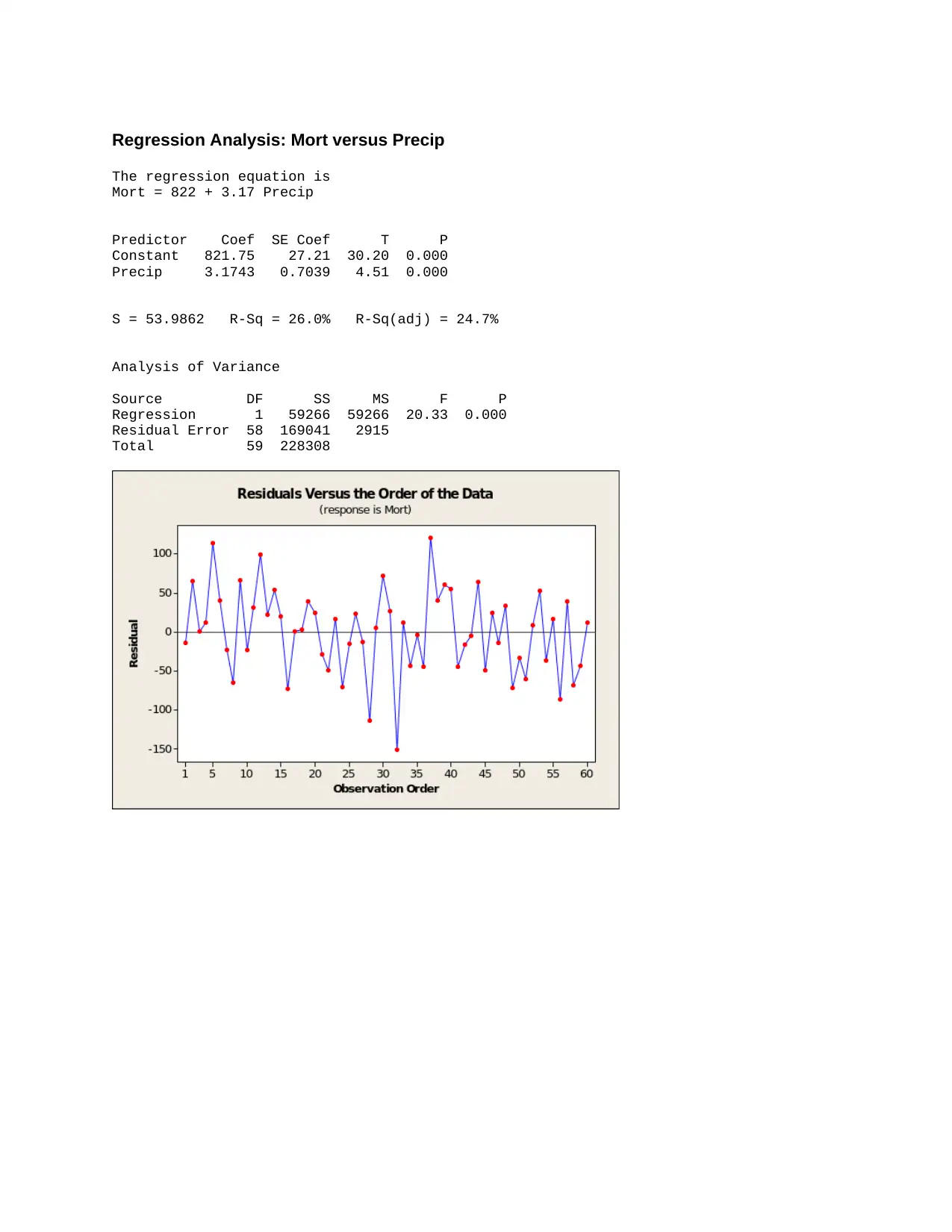
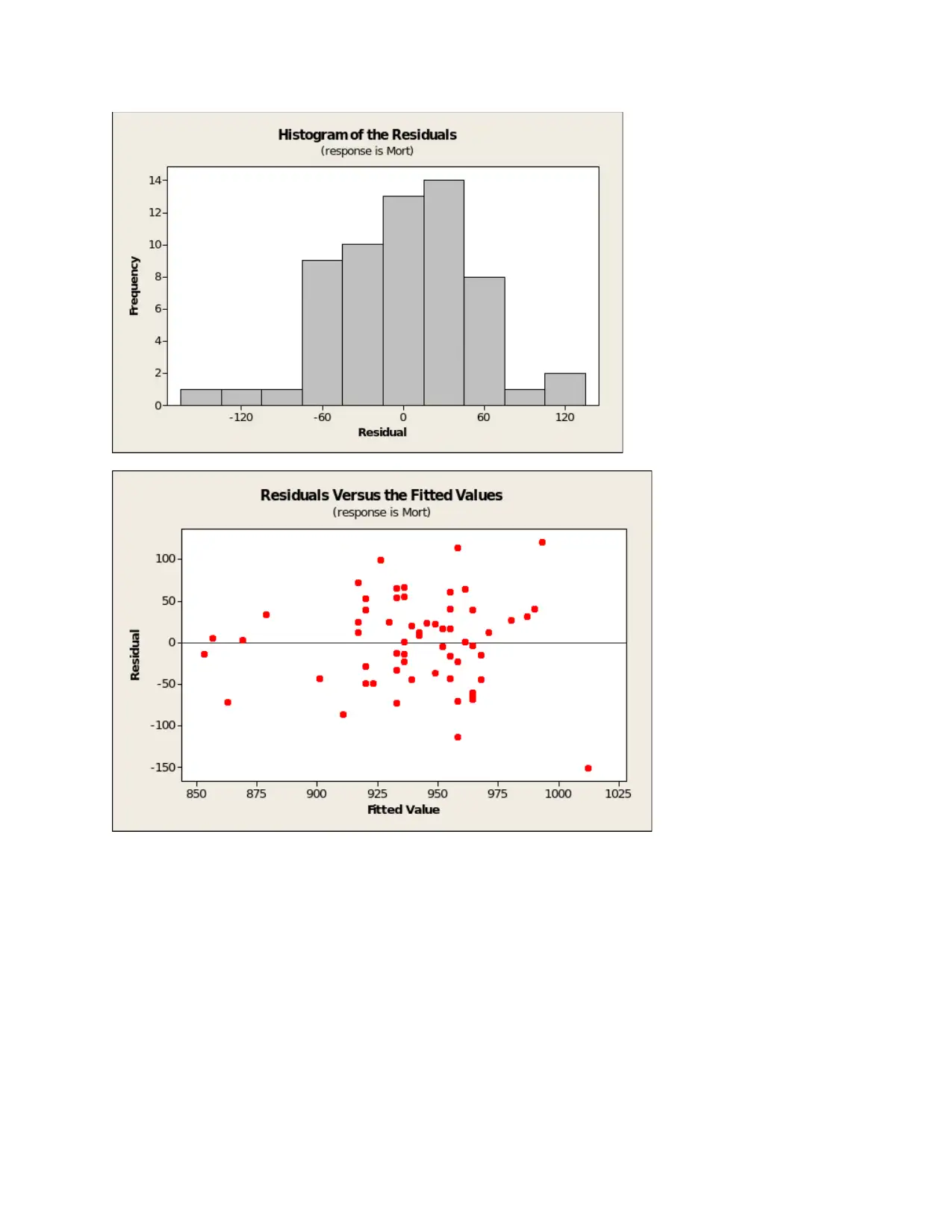
Regression Analysis: Mort versus Precip
The regression equation is
Mort = 822 + 3.17 Precip
Predictor Coef SE Coef T P
Constant 821.75 27.21 30.20 0.000
Precip 3.1743 0.7039 4.51 0.000
S = 53.9862 R-Sq = 26.0% R-Sq(adj) = 24.7%
Analysis of Variance
Source DF SS MS F P
Regression 1 59266 59266 20.33 0.000
Residual Error 58 169041 2915
Total 59 228308

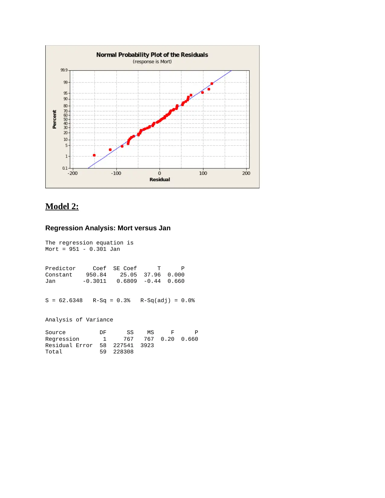
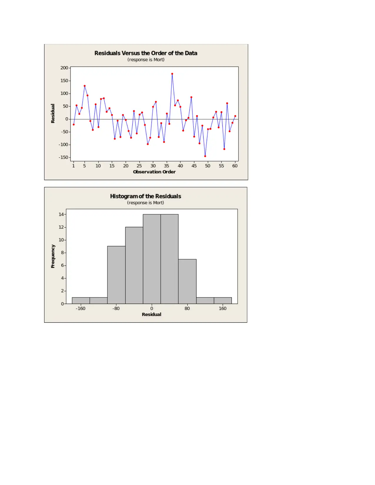
Model 2:
Regression Analysis: Mort versus Jan
The regression equation is
Mort = 951 - 0.301 Jan
Predictor Coef SE Coef T P
Constant 950.84 25.05 37.96 0.000
Jan -0.3011 0.6809 -0.44 0.660
S = 62.6348 R-Sq = 0.3% R-Sq(adj) = 0.0%
Analysis of Variance
Source DF SS MS F P
Regression 1 767 767 0.20 0.660
Residual Error 58 227541 3923
Total 59 228308

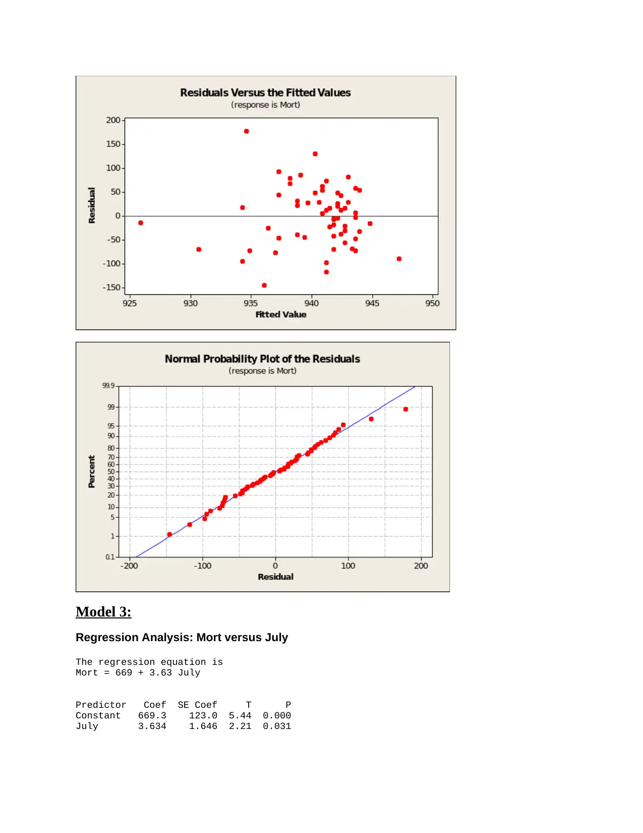
Model 3:
Regression Analysis: Mort versus July
The regression equation is
Mort = 669 + 3.63 July
Predictor Coef SE Coef T P
Constant 669.3 123.0 5.44 0.000
July 3.634 1.646 2.21 0.031

S = 60.2590 R-Sq = 7.8% R-Sq(adj) = 6.2%
Analysis of Variance
Source DF SS MS F P
Regression 1 17701 17701 4.87 0.031
Residual Error 58 210607 3631
Total 59 228308
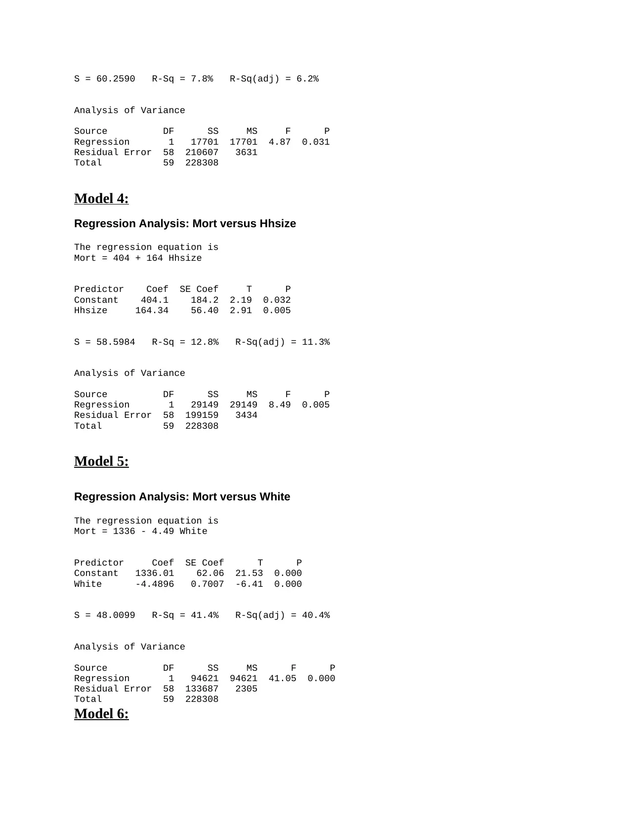
Model 4:
Regression Analysis: Mort versus Hhsize
The regression equation is
Mort = 404 + 164 Hhsize
Predictor Coef SE Coef T P
Constant 404.1 184.2 2.19 0.032
Hhsize 164.34 56.40 2.91 0.005
S = 58.5984 R-Sq = 12.8% R-Sq(adj) = 11.3%
Analysis of Variance
Source DF SS MS F P
Regression 1 29149 29149 8.49 0.005
Residual Error 58 199159 3434
Total 59 228308
Model 5:
Regression Analysis: Mort versus White
The regression equation is
Mort = 1336 - 4.49 White
Predictor Coef SE Coef T P
Constant 1336.01 62.06 21.53 0.000
White -4.4896 0.7007 -6.41 0.000
S = 48.0099 R-Sq = 41.4% R-Sq(adj) = 40.4%
Analysis of Variance
Source DF SS MS F P
Regression 1 94621 94621 41.05 0.000
Residual Error 58 133687 2305
Total 59 228308
Model 6:

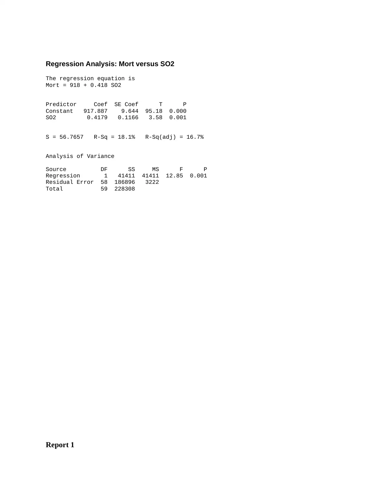
Regression Analysis: Mort versus SO2
The regression equation is
Mort = 918 + 0.418 SO2
Predictor Coef SE Coef T P
Constant 917.887 9.644 95.18 0.000
SO2 0.4179 0.1166 3.58 0.001
S = 56.7657 R-Sq = 18.1% R-Sq(adj) = 16.7%
Analysis of Variance
Source DF SS MS F P
Regression 1 41411 41411 12.85 0.001
Residual Error 58 186896 3222
Total 59 228308
Report 1

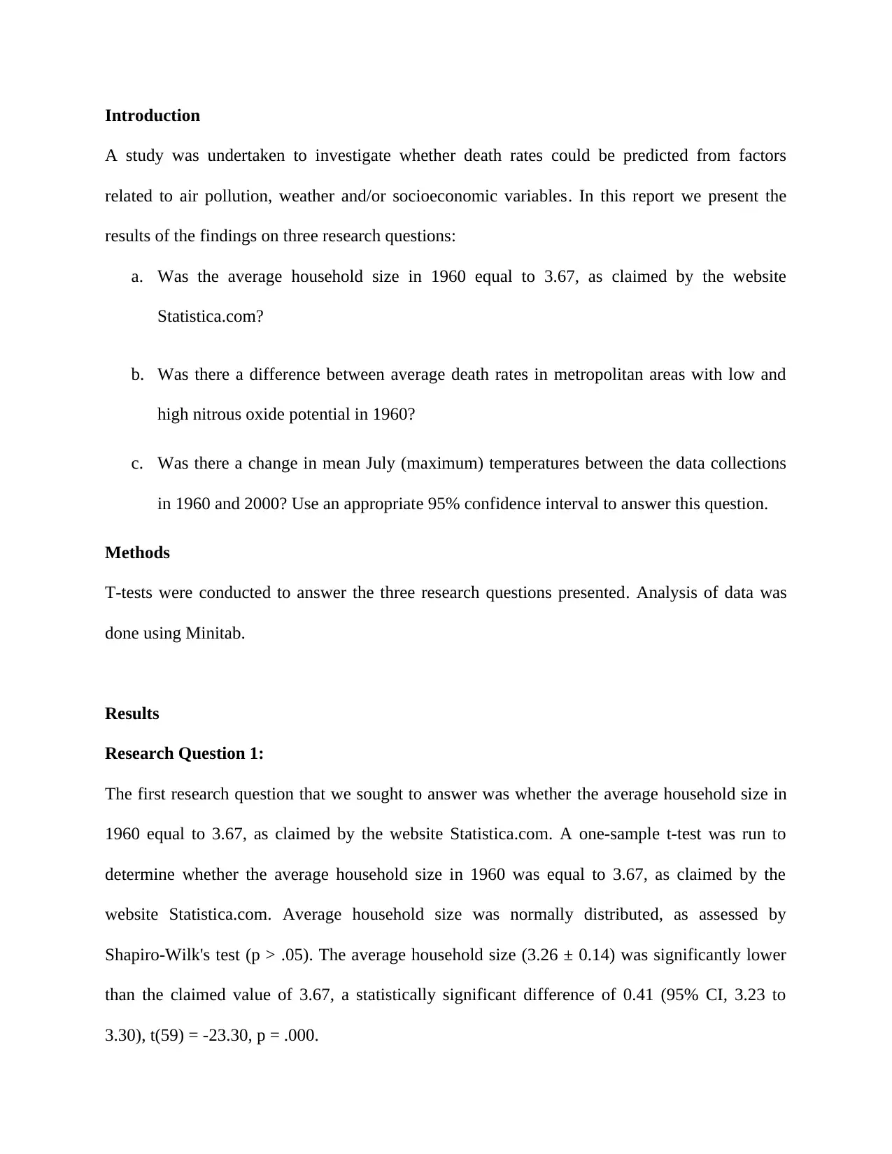
Introduction
A study was undertaken to investigate whether death rates could be predicted from factors
related to air pollution, weather and/or socioeconomic variables. In this report we present the
results of the findings on three research questions:
a. Was the average household size in 1960 equal to 3.67, as claimed by the website
Statistica.com?
b. Was there a difference between average death rates in metropolitan areas with low and
high nitrous oxide potential in 1960?
c. Was there a change in mean July (maximum) temperatures between the data collections
in 1960 and 2000? Use an appropriate 95% confidence interval to answer this question.
Methods
T-tests were conducted to answer the three research questions presented. Analysis of data was
done using Minitab.
Results
Research Question 1:
The first research question that we sought to answer was whether the average household size in
1960 equal to 3.67, as claimed by the website Statistica.com. A one-sample t-test was run to
determine whether the average household size in 1960 was equal to 3.67, as claimed by the
website Statistica.com. Average household size was normally distributed, as assessed by
Shapiro-Wilk's test (p > .05). The average household size (3.26 ± 0.14) was significantly lower
than the claimed value of 3.67, a statistically significant difference of 0.41 (95% CI, 3.23 to
3.30), t(59) = -23.30, p = .000.