IF2209 Derivatives Coursework: Analysis of Option Pricing Models
VerifiedAdded on 2023/06/15
|32
|6924
|137
Homework Assignment
AI Summary
This document presents a comprehensive solution to a derivatives coursework assignment, focusing on option pricing models and trading strategies. It begins with an analysis of put-call parity using linear regression to estimate parameters such as dividend yield and risk-free interest rate. The solution then delves into calculating implied volatility using the Black-Scholes-Merton model and Excel's Solver function, followed by an examination of the relationship between strike price and implied volatility, including quadratic fitting and outlier analysis. Furthermore, the coursework explores various option strategies like bull call spreads and seagull strategies, along with payoff calculations. The document also includes a two-period binomial model for European vanilla and digital options. The solution is supported by tables, figures, and regression analyses, providing a detailed and well-structured approach to understanding derivatives and option pricing. Desklib offers a wealth of similar solved assignments and past papers for students.

Page1 of32
Derivatives Coursework
Student Name: Student ID:
Unit Name: Unit ID:
Derivatives Coursework
Student Name: Student ID:
Unit Name: Unit ID:
Paraphrase This Document
Need a fresh take? Get an instant paraphrase of this document with our AI Paraphraser

Page2 of32
Table of tables
Table 1: Regression analysis including R ................................................................................................ 3
Table2: Strike vs Cobs-Pobs linear line fit plot ........................................................................................ 5
Table3: K residual plot for Cobs-Pobs values .......................................................................................... 5
Table 4: Solution table for σimpl for given K .......................................................................................... 7
Table 5:σimpl for given K ....................................................................................................................
Table6: σimplvs strike rate K plot ...........................................................................................................
Table 7:ANOVA for quadratic fit for table 3 data ................................................................................... 9
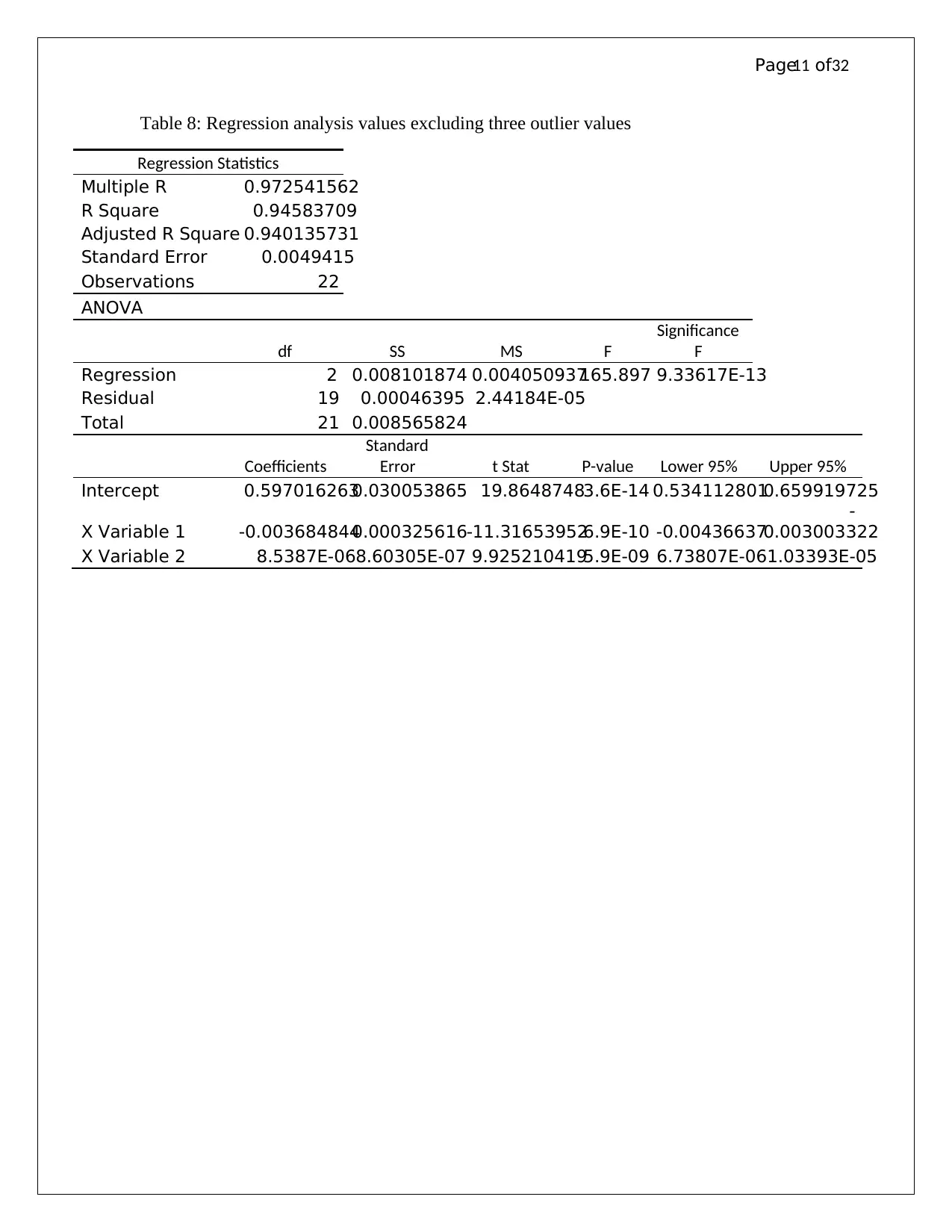
Table 8: Regression analysis values excluding three outlier values ....................................................... 11
Table 9: Bull Spread Strategy.................................................................................................................
Table 10: Bull Spread Payoff matrix ......................................................................................................
Table 11: Seagull strategy values ...........................................................................................................
Table 12: Seagull payoff values .............................................................................................................
Table 13: Short put butterflypayoff values ............................................................................................. 1
Table 14: Two-period binomial modelwith European vanilla payoff values ......................................... 19
Table 15: Two-period binomial modelwith Digital payoff values ......................................................... 21
Table 16: Regression Analysis for Question 1 with residual output ...................................................... 26
Table 17: Question 2 Solution for implied volatility .............................................................................. 28
Table 18: Regression Analysis for Question 2 with outliers .................................................................. 30
Table 19: Residual values with outliers for Question 2 .......................................................................... 31
Table 20: Regression Analysis for Question 2 without outliers ............................................................. 31
Table 21: Black Scholes calculation for Question 3 ............................................................................... 32
Table of figures
Figure 1: Scatter plot excluding outliers 10
Figure 2: Bull spread graph ...................................................................................................................
Figure 3: Seagull payoff graph ...............................................................................................................
Figure 4: Residual Plot for Question 1 ................................................................................................... 2
Table of tables
Table 1: Regression analysis including R ................................................................................................ 3
Table2: Strike vs Cobs-Pobs linear line fit plot ........................................................................................ 5
Table3: K residual plot for Cobs-Pobs values .......................................................................................... 5
Table 4: Solution table for σimpl for given K .......................................................................................... 7
Table 5:σimpl for given K ....................................................................................................................
Table6: σimplvs strike rate K plot ...........................................................................................................
Table 7:ANOVA for quadratic fit for table 3 data ................................................................................... 9
Table 8: Regression analysis values excluding three outlier values ....................................................... 11
Table 9: Bull Spread Strategy.................................................................................................................
Table 10: Bull Spread Payoff matrix ......................................................................................................
Table 11: Seagull strategy values ...........................................................................................................
Table 12: Seagull payoff values .............................................................................................................
Table 13: Short put butterflypayoff values ............................................................................................. 1
Table 14: Two-period binomial modelwith European vanilla payoff values ......................................... 19
Table 15: Two-period binomial modelwith Digital payoff values ......................................................... 21
Table 16: Regression Analysis for Question 1 with residual output ...................................................... 26
Table 17: Question 2 Solution for implied volatility .............................................................................. 28
Table 18: Regression Analysis for Question 2 with outliers .................................................................. 30
Table 19: Residual values with outliers for Question 2 .......................................................................... 31
Table 20: Regression Analysis for Question 2 without outliers ............................................................. 31
Table 21: Black Scholes calculation for Question 3 ............................................................................... 32
Table of figures
Figure 1: Scatter plot excluding outliers 10
Figure 2: Bull spread graph ...................................................................................................................
Figure 3: Seagull payoff graph ...............................................................................................................
Figure 4: Residual Plot for Question 1 ................................................................................................... 2

Page3 of32
ANS:1 Put-call parity requires that the following equation to hold
).....(....................0 iKeeSPC rTT
obsobs
−− −=− δ
• Where T=11 months
• obsobs PC , are observed prices of the call and put options
• δis continuously compounded dividend per year
• r is continuously compounded risk free interest per annum
• 0S is current spot price of the stock
• T is option maturity
Now linear regression general form of the equation is )........(.......... iixy βα+=
(i) Comparing equations (i) and (ii) it is obtained that rTT eeS −− −== βα δ ,0 where
KxPCy obsobs =−= ,
(ii) To fit the linear regression model, help of regression tool in excel has been used
Following results have been obtained:
Table 1: Regression analysis including R
Regression Statistics
Multiple R 0.997754
R Square 0.995512
Adjusted R Square 0.995368
Standard Error 3.5137
Observations 33
⊘ This is a preview!⊘
Do you want full access?
Subscribe today to unlock all pages.
Trusted by 1+ million students worldwide
Page4 of32
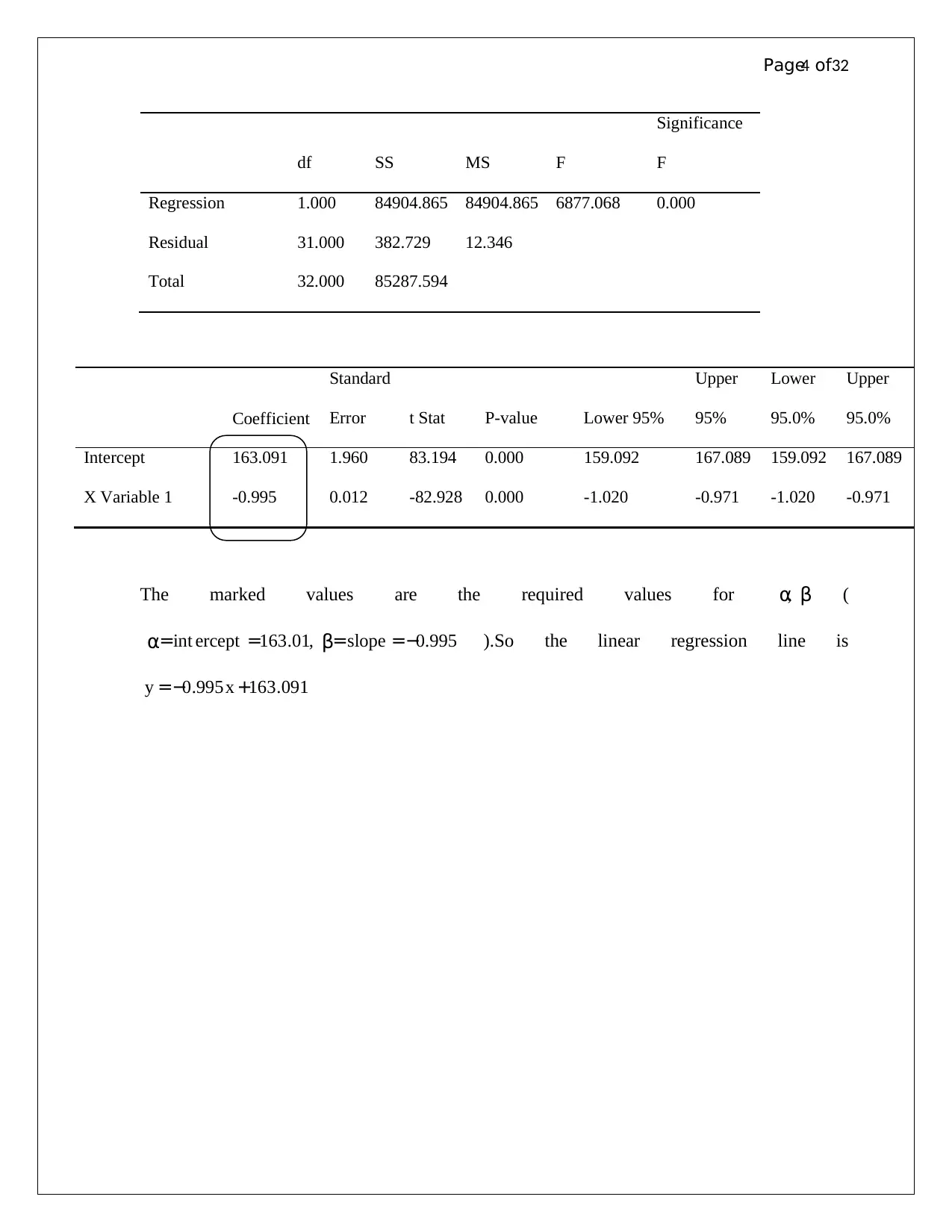
The marked values are the required values for βα, (
995.0,01.163int −==== slopeercept βα ).So the linear regression line is
091.163995.0 +−= xy
df SS MS F
Significance
F
Regression 1.000 84904.865 84904.865 6877.068 0.000
Residual 31.000 382.729 12.346
Total 32.000 85287.594
Coefficient
Standard
Error t Stat P-value Lower 95%
Upper
95%
Lower
95.0%
Upper
95.0%
Intercept 163.091 1.960 83.194 0.000 159.092 167.089 159.092 167.089
X Variable 1 -0.995 0.012 -82.928 0.000 -1.020 -0.971 -1.020 -0.971
Paraphrase This Document
Need a fresh take? Get an instant paraphrase of this document with our AI Paraphraser
Page5 of32
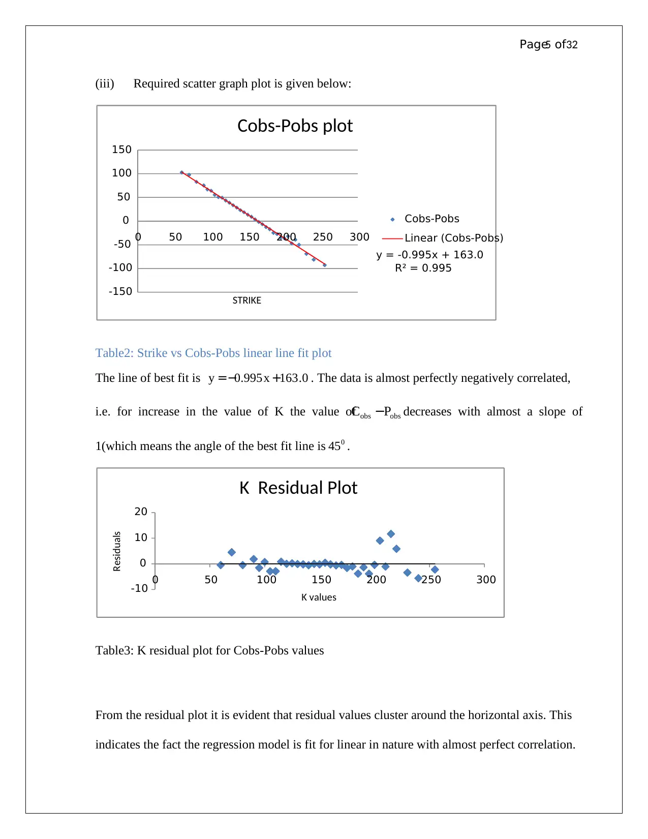
(iii) Required scatter graph plot is given below:
Table2: Strike vs Cobs-Pobs linear line fit plot
The line of best fit is 0.163995.0 +−= xy . The data is almost perfectly negatively correlated,
i.e. for increase in the value of K the value of obsobs PC − decreases with almost a slope of
1(which means the angle of the best fit line is 0
45 .
Table3: K residual plot for Cobs-Pobs values
From the residual plot it is evident that residual values cluster around the horizontal axis. This
indicates the fact the regression model is fit for linear in nature with almost perfect correlation.
y = -0.995x + 163.0
R² = 0.995
-150
-100
-50
0
50
100
150
0 50 100 150 200 250 300
STRIKE
Cobs-Pobs plot
Cobs-Pobs
Linear (Cobs-Pobs)
-10
0
10
20
0 50 100 150 200 250 300
Residuals
K values
K Residual Plot

Page6 of32
Now for 40.1650 =S and T=11/12, 995.0,01.163 −== βα following calculations can be
performed:
0158.0
40.165
01.163
ln*
11
12
ln*
1
ln
0
0
0
0
==>
−==>
−==>
=−>−=
==>
=
−
−
δ
δ
α
δ
α
δ
α
α
δ
δ
ST
S
T
e
S
eS
T
T
And
00547.0
)995.0ln(*
11
12
)ln(*
1
)ln(
==>
−==>
−=−=>
−=−=>
−= −
r
r
T
r
rT
e rT
β
β
β
Now for 40.1650 =S and T=11/12, 995.0,01.163 −== βα following calculations can be
performed:
0158.0
40.165
01.163
ln*
11
12
ln*
1
ln
0
0
0
0
==>
−==>
−==>
=−>−=
==>
=
−
−
δ
δ
α
δ
α
δ
α
α
δ
δ
ST
S
T
e
S
eS
T
T
And
00547.0
)995.0ln(*
11
12
)ln(*
1
)ln(
==>
−==>
−=−=>
−=−=>
−= −
r
r
T
r
rT
e rT
β
β
β
⊘ This is a preview!⊘
Do you want full access?
Subscribe today to unlock all pages.
Trusted by 1+ million students worldwide

Page7 of32
ANS:2 (a) Given values are δ = 1.53% per annum, r = 0.49% per annum, T = 11/12 year and
S0 = 165.40.
Black–Scholes–Merton formula gives the option price as:
( ) ( ) ( )2100 ,,,,, dNKedNeSTrKSC rTT
impBSM
−− −= δ
σδ
Where
+−−= Tr
K
S
T
d impl
impl
*
2
ln
1 2
0
1
σ
δ
σ
and Tdd impl *12 σ−= and ( ).N is the
standard normal cumulative distribution function.
The governing equation provided as ( ) )(..............................0,,,,,0 iTrKSCC impBSMobs =− σδ
Using Excel’s add-in solver equation (i) is solved and the solution is as follows:
Table 4: Solution table for σimpl for given K
K σimpl Cobs
115 27.200000 51.46
120 23.743192 46
125 39.400000 41.78
130 0.268155 37.4
135 0.252982 33
140 0.237571 28.68
145 0.245481 25.64
150 0.237140 22.05
155 0.242571 19.48
160 0.224743 15.8
165 0.220736 13.2
170 0.215498 10.8
175 0.207808 8.53
180 0.210950 7.18
185 0.205065 5.55
190 0.205596 4.5
195 0.198816 3.3
200 0.198853 2.6
205 0.199595 2.06
Paraphrase This Document
Need a fresh take? Get an instant paraphrase of this document with our AI Paraphraser
Page8 of32
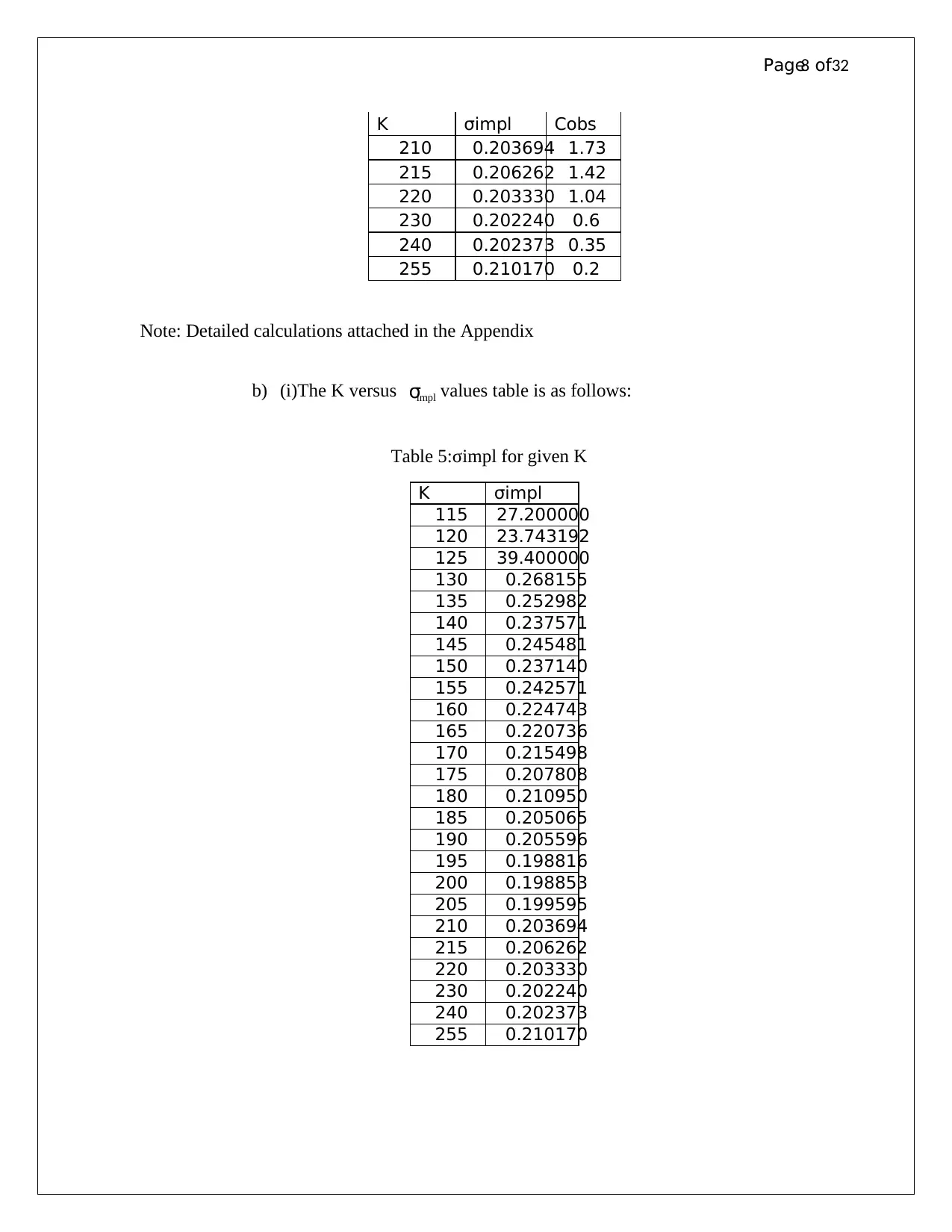
K σimpl Cobs
210 0.203694 1.73
215 0.206262 1.42
220 0.203330 1.04
230 0.202240 0.6
240 0.202373 0.35
255 0.210170 0.2
Note: Detailed calculations attached in the Appendix
b) (i)The K versus implσ values table is as follows:
Table 5:σimpl for given K
K σimpl
115 27.200000
120 23.743192
125 39.400000
130 0.268155
135 0.252982
140 0.237571
145 0.245481
150 0.237140
155 0.242571
160 0.224743
165 0.220736
170 0.215498
175 0.207808
180 0.210950
185 0.205065
190 0.205596
195 0.198816
200 0.198853
205 0.199595
210 0.203694
215 0.206262
220 0.203330
230 0.202240
240 0.202373
255 0.210170
Page9 of32
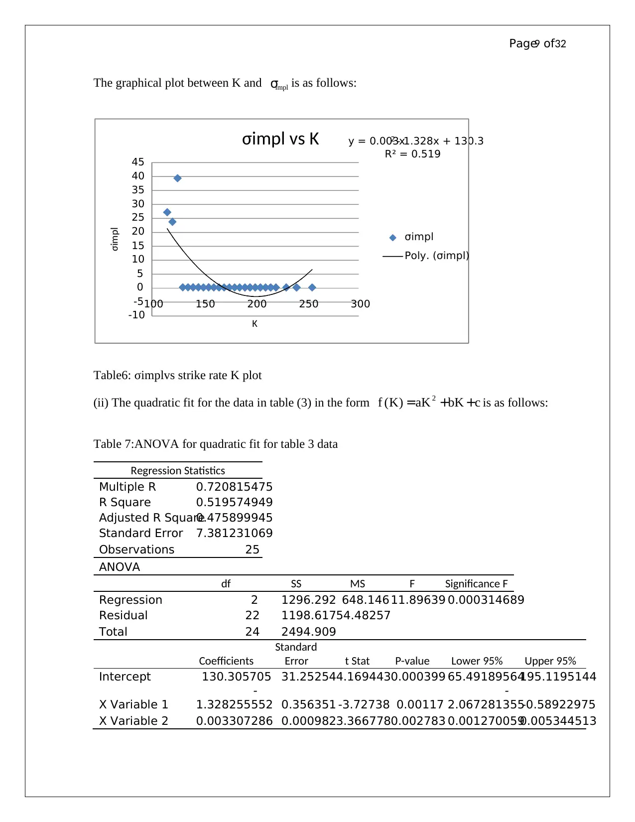
The graphical plot between K and implσ is as follows:
Table6: σimplvs strike rate K plot
(ii) The quadratic fit for the data in table (3) in the form cbKaKKf ++= 2
)( is as follows:
Table 7:ANOVA for quadratic fit for table 3 data
Regression Statistics
Multiple R 0.720815475
R Square 0.519574949
Adjusted R Square0.475899945
Standard Error 7.381231069
Observations 25
ANOVA
df SS MS F Significance F
Regression 2 1296.292 648.146 11.89639 0.000314689
Residual 22 1198.61754.48257
Total 24 2494.909
Coefficients
Standard
Error t Stat P-value Lower 95% Upper 95%
Intercept 130.305705 31.252544.1694430.000399 65.49189564195.1195144
X Variable 1
-
1.328255552 0.356351 -3.72738 0.00117
-
2.067281355-0.58922975
X Variable 2 0.003307286 0.0009823.3667780.002783 0.0012700590.005344513
y = 0.003x2 - 1.328x + 130.3
R² = 0.519
-10
-5
0
5
10
15
20
25
30
35
40
45
100 150 200 250 300
σimpl
K
σimpl vs K
σimpl
Poly. (σimpl)
⊘ This is a preview!⊘
Do you want full access?
Subscribe today to unlock all pages.
Trusted by 1+ million students worldwide

Page10 of32
From the ANOVA calculations it is evident that the intercept values are
305.130,328255.1,0033.0 === cba and the second order polynomial fit is
305.130328255.10033.0)( 2 ++= KKKf .
(iii) From table 2 it can be identified that three outlier values. Excluding them the trend of
the data is almost quadratic in nature and can be identified from the scatter plot.
Figure 1: Scatter plot excluding outliers
Excluding the outliers the regression analysis provides a well behaved intercept values.
y = 9E-06x2 - 0.003x + 0.597
R² = 0.945
0.150000
0.170000
0.190000
0.210000
0.230000
0.250000
0.270000
0.290000
0 50 100 150 200 250 300
σimpl
K
σimpl vs K
σimpl
Poly. (σimpl)
Paraphrase This Document
Need a fresh take? Get an instant paraphrase of this document with our AI Paraphraser
Page11 of32
Table 8: Regression analysis values excluding three outlier values
Regression Statistics
Multiple R 0.972541562
R Square 0.94583709
Adjusted R Square 0.940135731
Standard Error 0.0049415
Observations 22
ANOVA
df SS MS F
Significance
F
Regression 2 0.008101874 0.004050937165.897 9.33617E-13
Residual 19 0.00046395 2.44184E-05
Total 21 0.008565824
Coefficients
Standard
Error t Stat P-value Lower 95% Upper 95%
Intercept 0.5970162630.030053865 19.86487483.6E-14 0.5341128010.659919725
X Variable 1 -0.0036848440.000325616-11.316539526.9E-10 -0.00436637
-
0.003003322
X Variable 2 8.5387E-068.60305E-07 9.9252104195.9E-09 6.73807E-061.03393E-05

Page12 of32
ANS:3
(a) Given data values yearTKKyearryearS impl 1,80,70,/%8,/%35,70 210 ====== σ
Black–Scholes–Merton formula gives the option price as:
( ) ( ) ( )2100 ,,,,, dNKedNeSTrKSC rTT
impBSM
−− −= δ
σδ
Where
+−−= Tr
K
S
T
d impl
impl
*
2
ln
1 2
0
1
σ
δ
σ
and Tdd impl *12 σ−= and ( ).N is the
standard normal cumulative distribution function.
Now for 70=K ,
40357.0
1*
2
35.0*35.0
008.0
70
70
ln
1*35.0
1
1
1
==>
+−+=
d
d
Hence )05357.0(1*35.0040357.02 =−=d
So,
( ) ( ) ( )
)
(1282.12)05357.0(70040357.07035.0,1,0,08.0,70,70 08.00
value
timeNeNeC BSM =−= −−
Now for 80=K ,
022053.0
1*
2
35.0*35.0
008.0
80
70
ln
1*35.0
1
1
1
==>
+−+=
d
d
Hence )327946.0(1*35.0022053.02 =−=d
Now,
( ) ( ) ( )
)(
18.8)327946.0(80022053.07035.0,1,0,08.0,80,70 08.00
valuetime
NeNeC BSM =−= −−
Note: The C(BSM) value got evaluated in Excel using the above formulae.
⊘ This is a preview!⊘
Do you want full access?
Subscribe today to unlock all pages.
Trusted by 1+ million students worldwide
1 out of 32

Your All-in-One AI-Powered Toolkit for Academic Success.
+13062052269
info@desklib.com
Available 24*7 on WhatsApp / Email
![[object Object]](/_next/static/media/star-bottom.7253800d.svg)
Unlock your academic potential
Copyright © 2020–2026 A2Z Services. All Rights Reserved. Developed and managed by ZUCOL.