Descriptive Analytics and Visualization Report (Data Analysis)
VerifiedAdded on 2020/11/12
|21
|3008
|296
Report
AI Summary
This report presents a descriptive analytics and visualization analysis of insurance claims data. It utilizes Excel and SPSS to analyze various aspects of the data, including insurance claim conditions, sports and luxury vehicle savings, descriptive statistics of savings, customer approaches to insurers, and the average savings of different brokerage options (iChoose and uChoose). The analysis also examines customer satisfaction levels in rural and urban areas, comparing savings and providing graphical representations through histograms. Furthermore, the report investigates agreed and market values in relation to savings and explores the distribution of Diamond NCBR ratings among male and female customers. The findings are interpreted with statistical measures like mean, standard deviation, and proportions, providing insights into customer behavior and preferences related to insurance products.

Descriptive Analytics and Visualization
Paraphrase This Document
Need a fresh take? Get an instant paraphrase of this document with our AI Paraphraser
TABLE OF CONTENTS
INTRODUCTION...........................................................................................................................4
1...................................................................................................................................................4
2...................................................................................................................................................5
2.1 Sports.....................................................................................................................................5
2.2 Luxury....................................................................................................................................6
3. Descriptive statistics of savings ..............................................................................................6
4. .................................................................................................................................................7
5. .................................................................................................................................................7
6...................................................................................................................................................8
7...................................................................................................................................................8
Urban population ........................................................................................................................9
8.................................................................................................................................................11
APPENDIX....................................................................................................................................13
1.................................................................................................................................................13
2.................................................................................................................................................13
2.1..............................................................................................................................................14
3.................................................................................................................................................15
5.................................................................................................................................................16
7.a...............................................................................................................................................18
7.2..............................................................................................................................................20

⊘ This is a preview!⊘
Do you want full access?
Subscribe today to unlock all pages.
Trusted by 1+ million students worldwide
INTRODUCTION
Descriptive analytic and visualization plays very efficient role for analyzing any specific
data set along with proper interpretation and conclusion. The present report would be conveying
its findings with proper understanding. It would be also articulating proper application of
quantitative reasoning skills for the purpose of solving various complex problems. In the same
series, it would be also justifying various technologies for finding and disseminate information.
Further it had articulated different solutions for problems which are authentic. It had also
reflected understanding on data analysis which is contemporary and tools of visualization for
recognizing information of these tools. It would be using various tools from excel and SPSS with
preoper calculations.
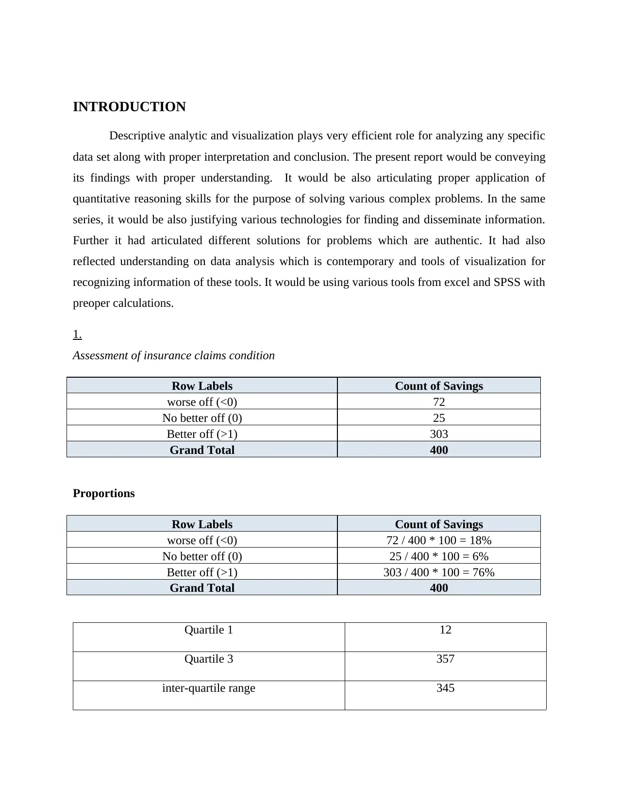
1.
Assessment of insurance claims condition
Row Labels Count of Savings
worse off (<0) 72
No better off (0) 25
Better off (>1) 303
Grand Total 400
Proportions
Row Labels Count of Savings
worse off (<0) 72 / 400 * 100 = 18%
No better off (0) 25 / 400 * 100 = 6%
Better off (>1) 303 / 400 * 100 = 76%
Grand Total 400
Quartile 1 12
Quartile 3 357
inter-quartile range 345
Descriptive analytic and visualization plays very efficient role for analyzing any specific
data set along with proper interpretation and conclusion. The present report would be conveying
its findings with proper understanding. It would be also articulating proper application of
quantitative reasoning skills for the purpose of solving various complex problems. In the same
series, it would be also justifying various technologies for finding and disseminate information.
Further it had articulated different solutions for problems which are authentic. It had also
reflected understanding on data analysis which is contemporary and tools of visualization for
recognizing information of these tools. It would be using various tools from excel and SPSS with
preoper calculations.
1.
Assessment of insurance claims condition
Row Labels Count of Savings
worse off (<0) 72
No better off (0) 25
Better off (>1) 303
Grand Total 400
Proportions
Row Labels Count of Savings
worse off (<0) 72 / 400 * 100 = 18%
No better off (0) 25 / 400 * 100 = 6%
Better off (>1) 303 / 400 * 100 = 76%
Grand Total 400
Quartile 1 12
Quartile 3 357
inter-quartile range 345
Paraphrase This Document
Need a fresh take? Get an instant paraphrase of this document with our AI Paraphraser
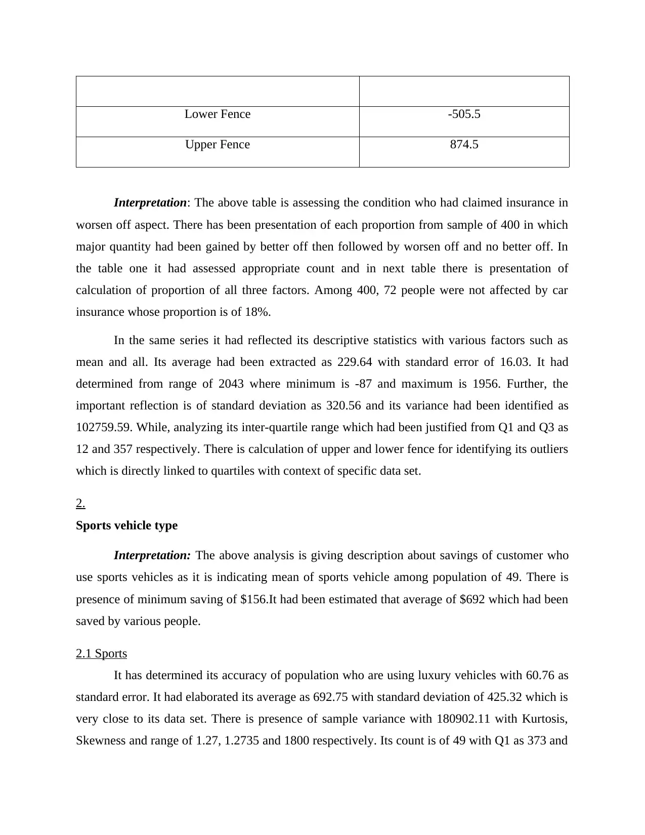
Lower Fence -505.5
Upper Fence 874.5
Interpretation: The above table is assessing the condition who had claimed insurance in
worsen off aspect. There has been presentation of each proportion from sample of 400 in which
major quantity had been gained by better off then followed by worsen off and no better off. In
the table one it had assessed appropriate count and in next table there is presentation of
calculation of proportion of all three factors. Among 400, 72 people were not affected by car
insurance whose proportion is of 18%.
In the same series it had reflected its descriptive statistics with various factors such as
mean and all. Its average had been extracted as 229.64 with standard error of 16.03. It had
determined from range of 2043 where minimum is -87 and maximum is 1956. Further, the
important reflection is of standard deviation as 320.56 and its variance had been identified as
102759.59. While, analyzing its inter-quartile range which had been justified from Q1 and Q3 as
12 and 357 respectively. There is calculation of upper and lower fence for identifying its outliers
which is directly linked to quartiles with context of specific data set.
2.
Sports vehicle type
Interpretation: The above analysis is giving description about savings of customer who
use sports vehicles as it is indicating mean of sports vehicle among population of 49. There is
presence of minimum saving of $156.It had been estimated that average of $692 which had been
saved by various people.
2.1 Sports
It has determined its accuracy of population who are using luxury vehicles with 60.76 as
standard error. It had elaborated its average as 692.75 with standard deviation of 425.32 which is
very close to its data set. There is presence of sample variance with 180902.11 with Kurtosis,
Skewness and range of 1.27, 1.2735 and 1800 respectively. Its count is of 49 with Q1 as 373 and
Q3 as 850. These quartile has helped in identifying lower and upper fence with tukey rule as -
342.5 and 1565.5 respectively.
2.2 Luxury
In the same series, it had justified its level of accuracy of population which are using
sports vehicle as 38.83 as its mean 507.19 helps in deviating from population's actual mean. In
simple words, it could be justified with value of data set which is very close to its mean as
274.29 as standard deviation. It has extracted its sample variance as 75235.61 which helps in
measuring that how far of set of numbers which is known as spread with value of average. The
median of data set is 417.5 is used for determining quartile 1 as middle number among smallest
and median. In the same series, its Q3 is 637.25 as middle number between data set's highest
value and middle value. From tukey's rule it had extracted it had determined its outliers for
setting limit of various data scores. Its lower is -110.87 with upper fence of 1086.125.
Luxury vehicle type
Interpretation: The above analysis is giving description about savings of customer who
use luxury vehicles. It had been estimated that 62 people are using luxury vehicles among the
selected sample. It had been indicated that they save average of $507.92 which is considered as
good indicator.
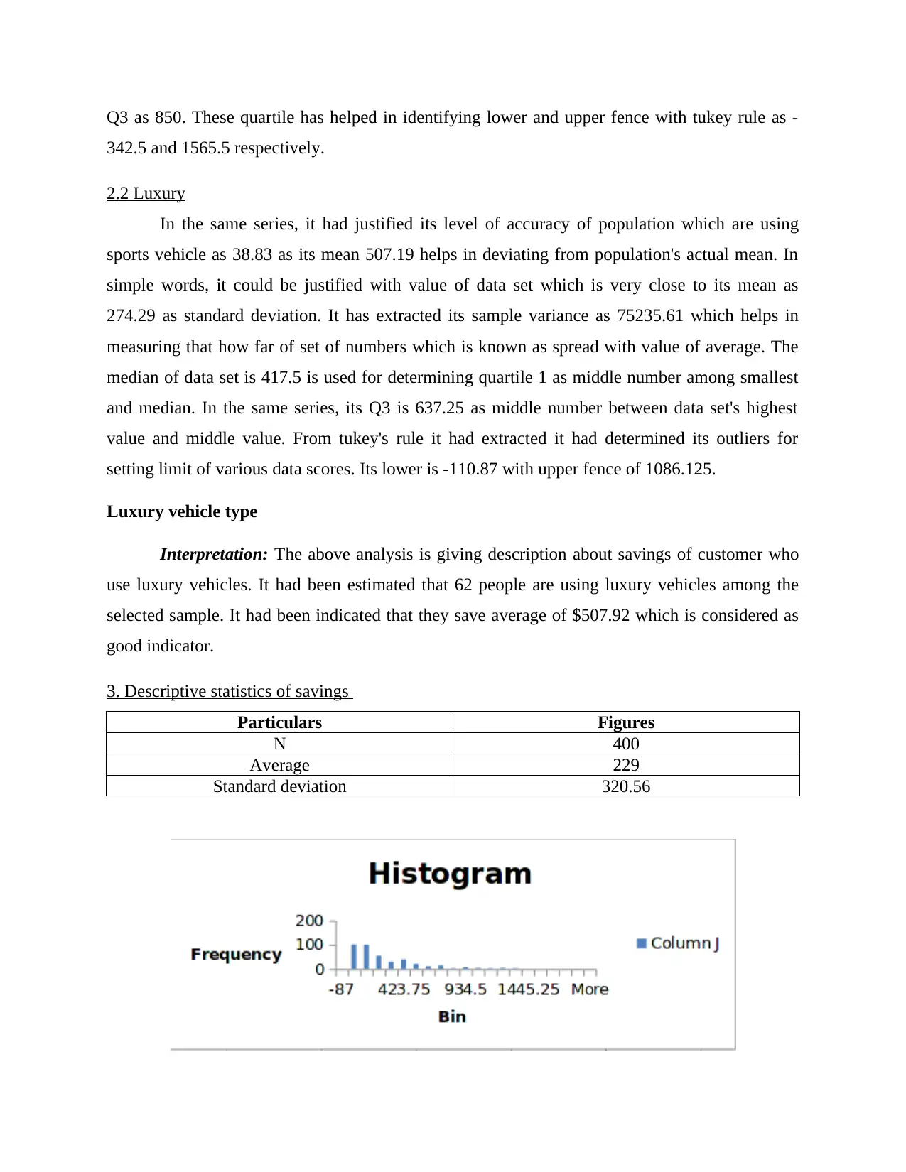
3. Descriptive statistics of savings
Particulars Figures
N 400
Average 229
Standard deviation 320.56
342.5 and 1565.5 respectively.
2.2 Luxury
In the same series, it had justified its level of accuracy of population which are using
sports vehicle as 38.83 as its mean 507.19 helps in deviating from population's actual mean. In
simple words, it could be justified with value of data set which is very close to its mean as
274.29 as standard deviation. It has extracted its sample variance as 75235.61 which helps in
measuring that how far of set of numbers which is known as spread with value of average. The
median of data set is 417.5 is used for determining quartile 1 as middle number among smallest
and median. In the same series, its Q3 is 637.25 as middle number between data set's highest
value and middle value. From tukey's rule it had extracted it had determined its outliers for
setting limit of various data scores. Its lower is -110.87 with upper fence of 1086.125.
Luxury vehicle type
Interpretation: The above analysis is giving description about savings of customer who
use luxury vehicles. It had been estimated that 62 people are using luxury vehicles among the
selected sample. It had been indicated that they save average of $507.92 which is considered as
good indicator.
3. Descriptive statistics of savings
Particulars Figures
N 400
Average 229
Standard deviation 320.56
⊘ This is a preview!⊘
Do you want full access?
Subscribe today to unlock all pages.
Trusted by 1+ million students worldwide
Interpretation: The above table is depicting actual figure which had been saved in
present scenario. The average savings were at least $260 on premium of car insurance but by
analyzing it from descriptive statistics it is justified as approx 230 of average saving whose
standard deviation is extracted as 16.02 with count of 400.
4.
Approached Insurer
No 340 85%
Yes 60 15%
Total Result 400
The above table is indicating proportion of customers for negotiating a better deal with
their insurance company as compared to approaching an insurer. There is aggregate population
of 400 in which 15% of 60 are approaching insurer and rest 85% are not approaching. Hence, it
is tested that less than 20% are contacting broker for negotiating better deal.
5.
Average of ichoose and uChoose
Broker
iChoose $262.44
uChoose $230.85
Total Result $253.76
From this specific analysis it could be concluded that average of ichoose had saved
average of 262.44 on the context of premium of insurance. There is calculation of broker
uChoose which is interpreting its average as 230.84 on premium of insurance of car.
Paraphrase This Document
Need a fresh take? Get an instant paraphrase of this document with our AI Paraphraser
Descriptive statistics of ichoose
The descriptive statistics is used for extracting average savings of ichoose has been
interpreted as 262.44 with its accuracy as 127282 with median of 127. It also helps in reflecting
its standard deviation as 356.76 with specific count of 190. In the same series, mean of savings
of uchoose is replicated as 230.85.
6.
1 2
Total Count of Customer
dissatisfaction
Row
Labels
Count of Customer
dissatisfaction
Count of Customer
dissatisfaction
Dissatisf
ied 33 59 92
Grand
Total 33 59 92
Proportion of customer’s dissatisfaction (In Rural area): 33 / 92 * 100
= 35.9%
Proportion of customer’s dissatisfaction (In Urban area): 59 / 92* 100
= 64.1%
In the above table it had been justified that in rural population, 33 were dissatisfied and
against to it urban population was quite double to approx 59. It has been interpreted through
pivot table of rural and urban population.
7.
(a) The average savings of rural and urban had been presented in below mentioned table:
Variable Average Savings
Rural 193.3157
Urban 240.9537
Urban population
Interpretation: The above graph is depicting histogram of savings of urban population
with its descriptive statistics. It had been justified that its average saving is of 240.95 with its
standard deviation of 19.06 as its accuracy is of 110913 with count of 305 along with range of
2034.
Rural population
Interpretation: The above graph is depicting average savings of rural population with its
descriptive statistics. The average saving is of 193.31 with accuracy of 75735.8. It had been
justified that its count is of 95 with standard deviation of 275.201 which is near to its observing
mean value.
⊘ This is a preview!⊘
Do you want full access?
Subscribe today to unlock all pages.
Trusted by 1+ million students worldwide
It could be justified that, average savings of both rural has huge variation. Sample 1 is
indicating population of rural and sample 2 as urban. The population which belongs to rural has
average saving of 193.31 and on its contrary, urban population has 240.9537.
(b)
Val_Method
Agreed Value $360.64
Market Value $213.45
Total Result $229.64
Histogram of agreed value
Interpretation: The above graph is justifying average saving of agreed value with 360.3
as its level of accuracy is 175218 with count of 44. The above graph is histogram of savings
related to agreed value. It had represented its maximum level of 1651 with minimum of -76. It
had represented its 6 bins with appropriate representation of graph.
Histogram of market value
Paraphrase This Document
Need a fresh take? Get an instant paraphrase of this document with our AI Paraphraser
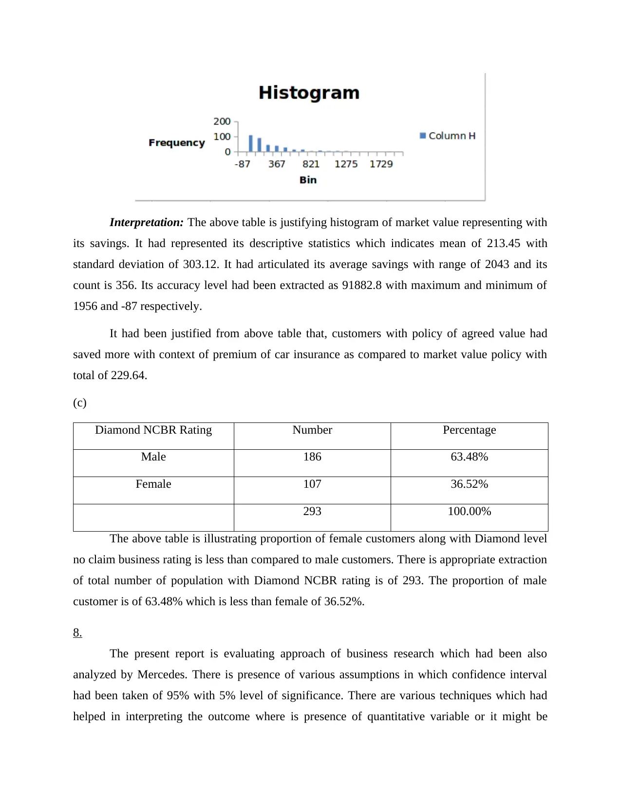
Interpretation: The above table is justifying histogram of market value representing with
its savings. It had represented its descriptive statistics which indicates mean of 213.45 with
standard deviation of 303.12. It had articulated its average savings with range of 2043 and its
count is 356. Its accuracy level had been extracted as 91882.8 with maximum and minimum of
1956 and -87 respectively.
It had been justified from above table that, customers with policy of agreed value had
saved more with context of premium of car insurance as compared to market value policy with
total of 229.64.
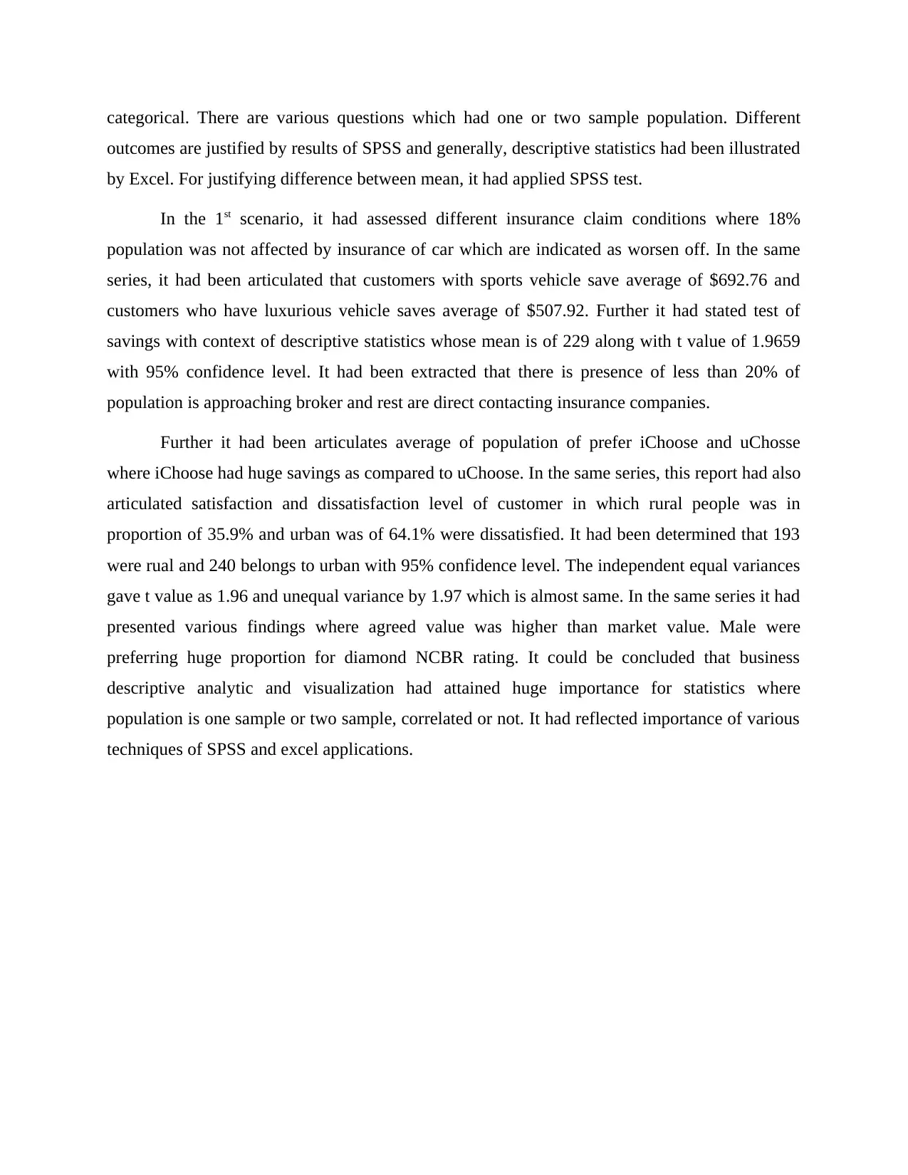
(c)
Diamond NCBR Rating Number Percentage
Male 186 63.48%
Female 107 36.52%
293 100.00%
The above table is illustrating proportion of female customers along with Diamond level
no claim business rating is less than compared to male customers. There is appropriate extraction
of total number of population with Diamond NCBR rating is of 293. The proportion of male
customer is of 63.48% which is less than female of 36.52%.
8.
The present report is evaluating approach of business research which had been also
analyzed by Mercedes. There is presence of various assumptions in which confidence interval
had been taken of 95% with 5% level of significance. There are various techniques which had
helped in interpreting the outcome where is presence of quantitative variable or it might be
its savings. It had represented its descriptive statistics which indicates mean of 213.45 with
standard deviation of 303.12. It had articulated its average savings with range of 2043 and its
count is 356. Its accuracy level had been extracted as 91882.8 with maximum and minimum of
1956 and -87 respectively.
It had been justified from above table that, customers with policy of agreed value had
saved more with context of premium of car insurance as compared to market value policy with
total of 229.64.
(c)
Diamond NCBR Rating Number Percentage
Male 186 63.48%
Female 107 36.52%
293 100.00%
The above table is illustrating proportion of female customers along with Diamond level
no claim business rating is less than compared to male customers. There is appropriate extraction
of total number of population with Diamond NCBR rating is of 293. The proportion of male
customer is of 63.48% which is less than female of 36.52%.
8.
The present report is evaluating approach of business research which had been also
analyzed by Mercedes. There is presence of various assumptions in which confidence interval
had been taken of 95% with 5% level of significance. There are various techniques which had
helped in interpreting the outcome where is presence of quantitative variable or it might be
categorical. There are various questions which had one or two sample population. Different
outcomes are justified by results of SPSS and generally, descriptive statistics had been illustrated
by Excel. For justifying difference between mean, it had applied SPSS test.
In the 1st scenario, it had assessed different insurance claim conditions where 18%
population was not affected by insurance of car which are indicated as worsen off. In the same
series, it had been articulated that customers with sports vehicle save average of $692.76 and
customers who have luxurious vehicle saves average of $507.92. Further it had stated test of
savings with context of descriptive statistics whose mean is of 229 along with t value of 1.9659
with 95% confidence level. It had been extracted that there is presence of less than 20% of
population is approaching broker and rest are direct contacting insurance companies.
Further it had been articulates average of population of prefer iChoose and uChosse
where iChoose had huge savings as compared to uChoose. In the same series, this report had also
articulated satisfaction and dissatisfaction level of customer in which rural people was in
proportion of 35.9% and urban was of 64.1% were dissatisfied. It had been determined that 193
were rual and 240 belongs to urban with 95% confidence level. The independent equal variances
gave t value as 1.96 and unequal variance by 1.97 which is almost same. In the same series it had
presented various findings where agreed value was higher than market value. Male were
preferring huge proportion for diamond NCBR rating. It could be concluded that business
descriptive analytic and visualization had attained huge importance for statistics where
population is one sample or two sample, correlated or not. It had reflected importance of various
techniques of SPSS and excel applications.
⊘ This is a preview!⊘
Do you want full access?
Subscribe today to unlock all pages.
Trusted by 1+ million students worldwide
1 out of 21

Your All-in-One AI-Powered Toolkit for Academic Success.
+13062052269
info@desklib.com
Available 24*7 on WhatsApp / Email
![[object Object]](/_next/static/media/star-bottom.7253800d.svg)
Unlock your academic potential
Copyright © 2020–2026 A2Z Services. All Rights Reserved. Developed and managed by ZUCOL.