MAE256 T2 2017 Assignment: Regression Analysis of House Sale Data
VerifiedAdded on 2020/02/24
|12
|1339
|190
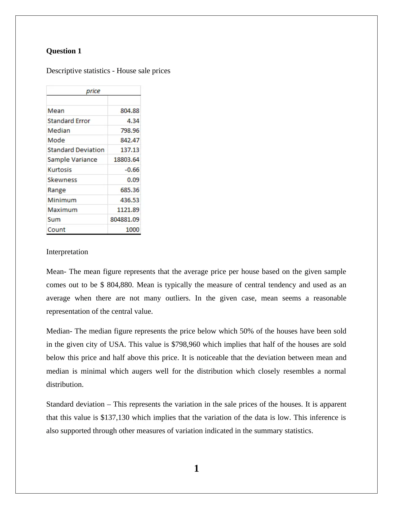
Homework Assignment
AI Summary
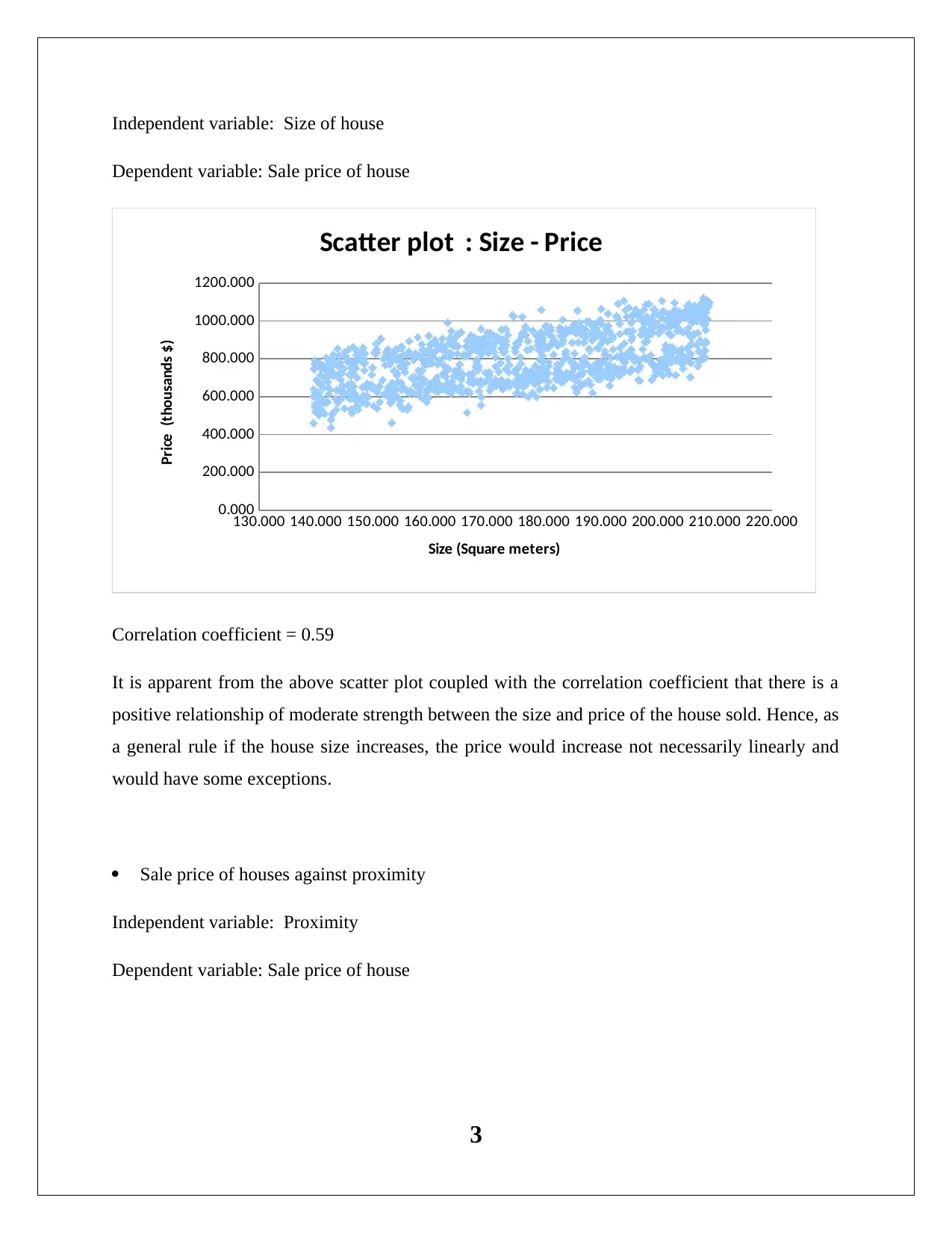
This document presents a comprehensive solution to a statistics assignment (MAE256 T2 2017) focusing on the analysis of house sale prices. The solution begins with descriptive statistics, including the interpretation of mean, median, standard deviation, and skewness. It then explores the relationship between house prices and various factors such as size and proximity to the central business district (CBD) using correlation coefficients and scatter plots. The assignment delves into linear regression models, examining the impact of size, age, and proximity on house prices, and also incorporates dummy variables for features like pools and fireplaces. Furthermore, it investigates the use of logarithmic transformations and hypothesis testing to assess the statistical significance of different variables on house sale prices. The solution concludes with an analysis of the joint significance of the regression model through ANOVA and F-tests.
1 out of 12
Related Documents


Your All-in-One AI-Powered Toolkit for Academic Success.
+13062052269
info@desklib.com
Available 24*7 on WhatsApp / Email
![[object Object]](/_next/static/media/star-bottom.7253800d.svg)
Copyright © 2020–2026 A2Z Services. All Rights Reserved. Developed and managed by ZUCOL.