University Design Optimisation for Manufacturing Project Report

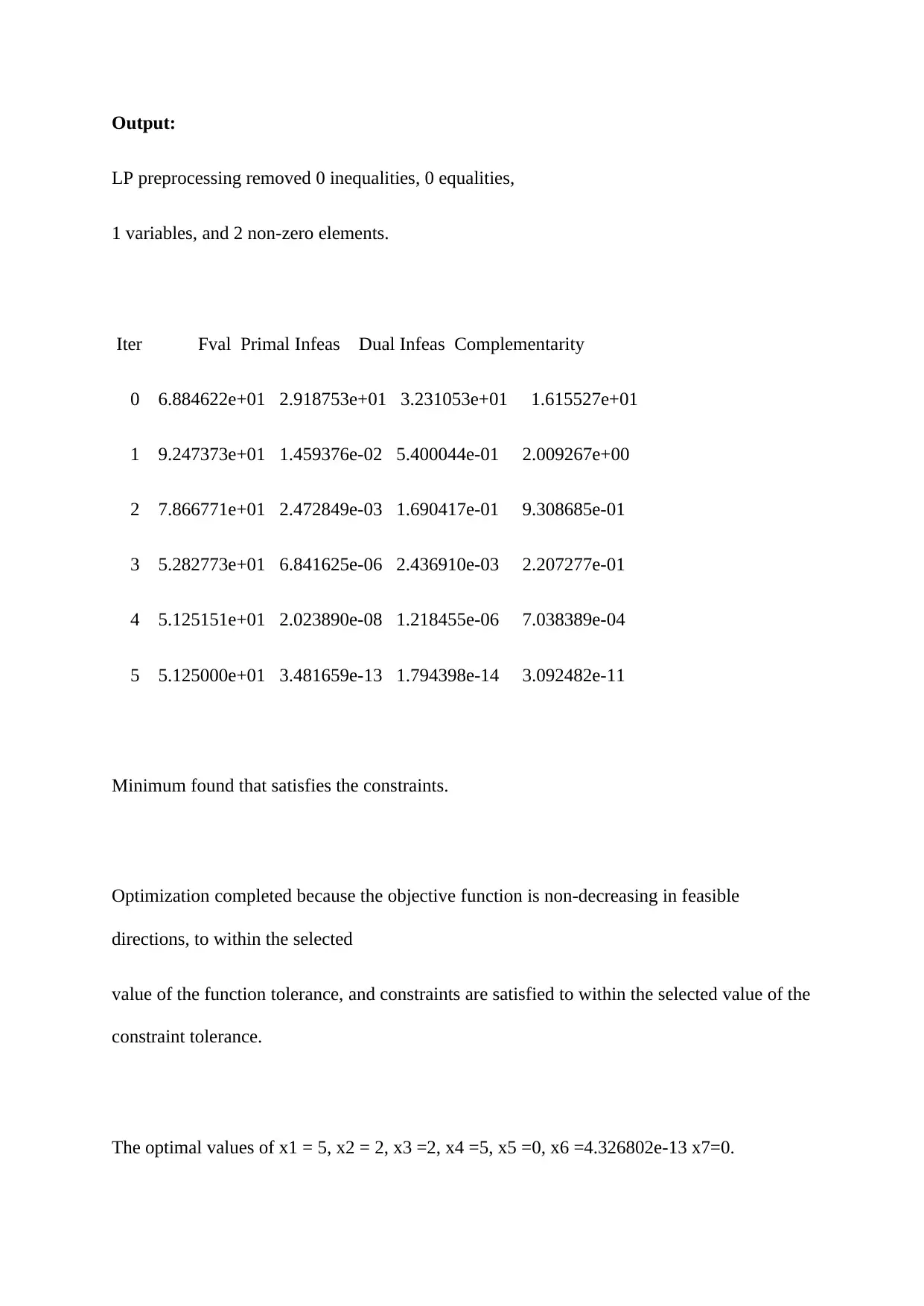
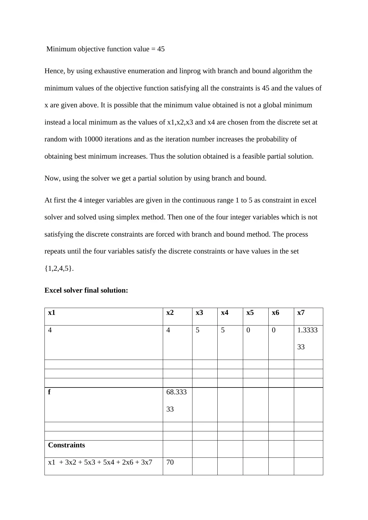
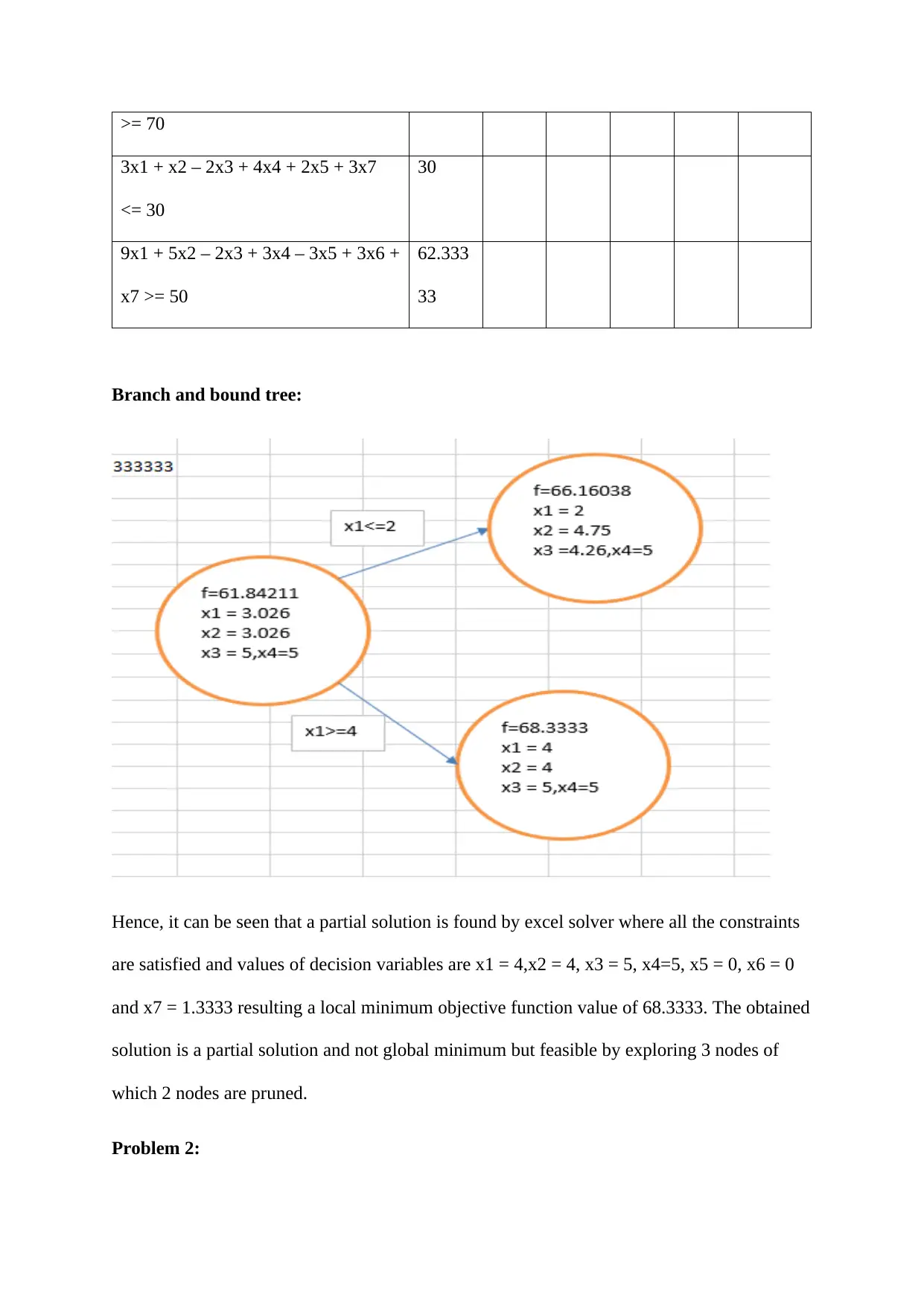
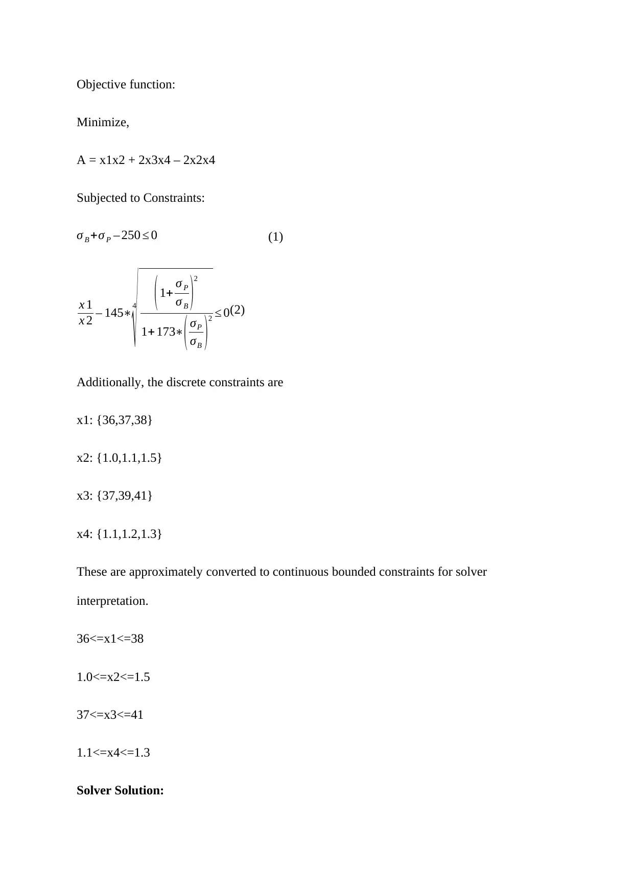
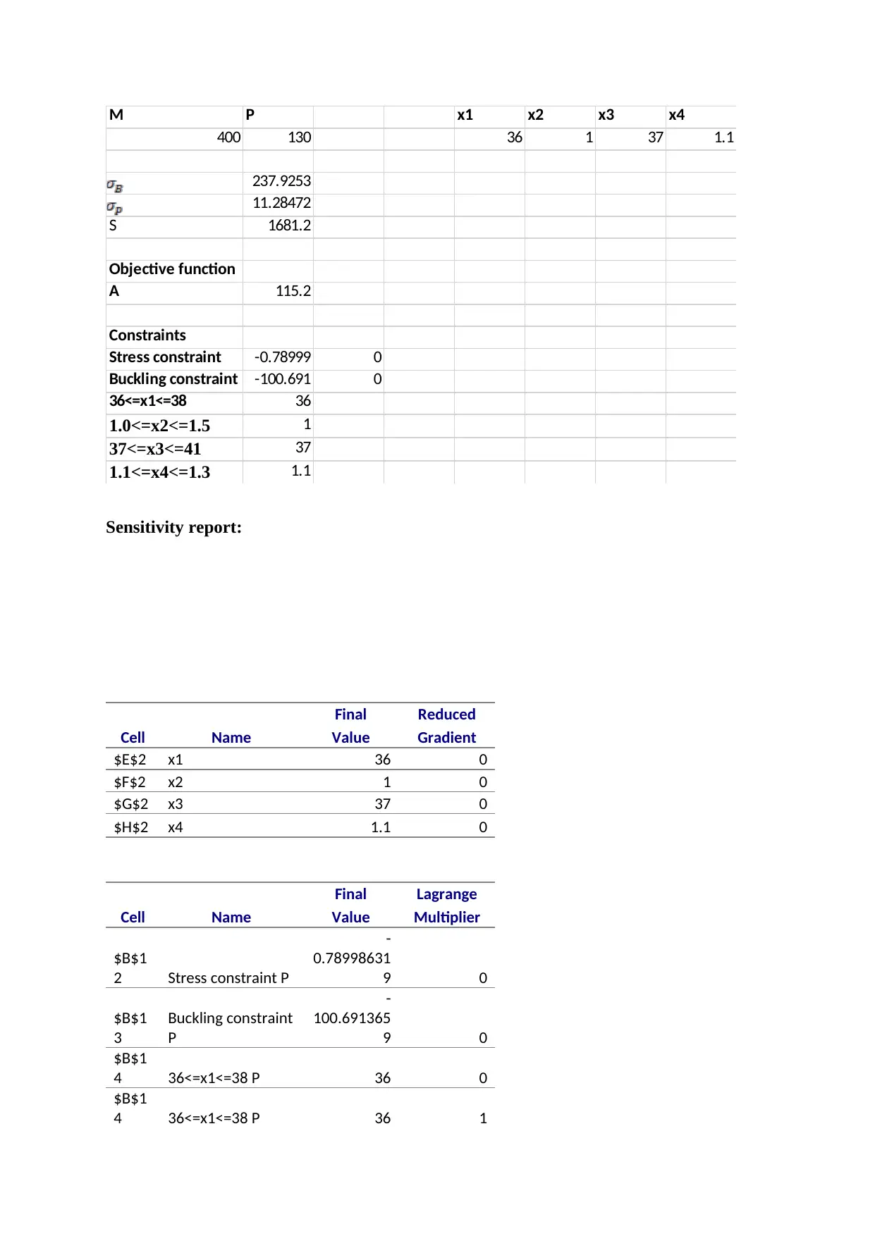
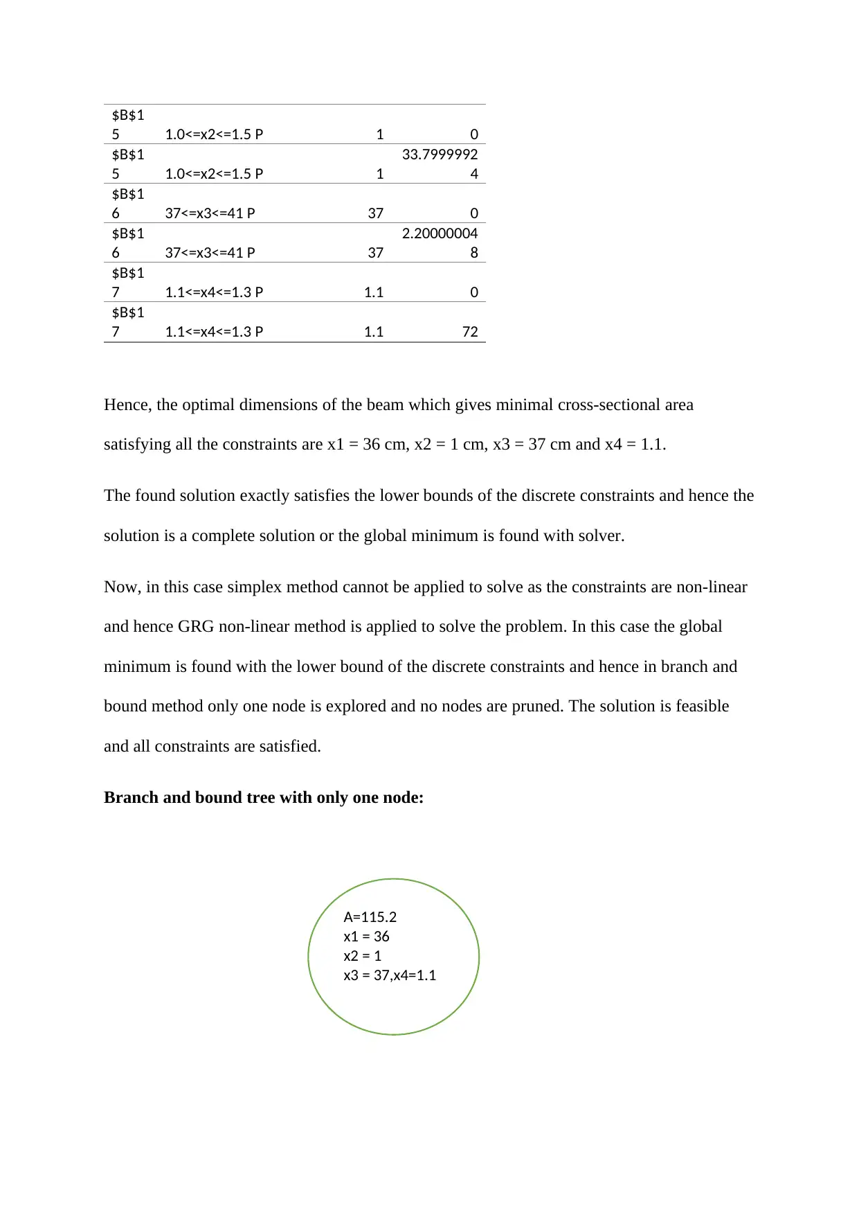
This project report presents solutions to two design optimisation problems for manufacturing, addressing both mixed-integer linear and discrete nonlinear optimisation scenarios. The first problem is solved using exhaustive enumeration and linear programming (linprog) in MATLAB, along with branch and bound techniques using linprog and Excel Solver. The second problem employs a solver solution, utilizing GRG non-linear method due to the non-linear constraints, and explores the branch and bound method. The report includes MATLAB code, solver outputs, branch and bound trees, and sensitivity reports to demonstrate the solution process and results. The report evaluates the solutions' efficiency and identifies partial and complete solutions, including the optimal values of the decision variables and the minimum objective function values, providing a detailed analysis of the optimisation processes.

DESIGN OPTIMISATION FOR MANUFACTURING
DESIGN OPTIMISATION FOR MANUFACTURING
Name of the Student
Name of the University
Author Note

Problem 1:
Minimise:
f = 2x1 + 6x2 + 4x3 + 3x4 + 2*x5 + 6*x6 + x7
Subject to:
x1 + 3x2 + 5x3 + 5x4 + 2x6 + 3x7 >= 70
3x1 + x2 – 2x3 + 4x4 + 2x5 + 3x7 <= 30
9x1 + 5x2 – 2x3 + 3x4 – 3x5 + 3x6 + x7 >= 50
x1,x2,x3,x4 ∈ {1,2,4,5}
x5, x6, x7 >= 0
Now, for using exhaustive enumeration the discrete variables are considered and continuous
variables are made to zero.
Minimise:
f = 2x1 + 6x2 + 4x3 + 3x4
Subjected to the same constraints as above.
MATLAB code:
clc
clear
f = [2 6 4 3 2 6 1];
A = [-1 -3 -5 -5 0 -2 -3
3 1 -2 4 2 0 3

-9 -5 2 -3 3 -3 -1];
b = [-70 30 -50];
lb = zeros(1,length(f));
%%% Initially continuous variable are set to zero
x5 = 0; x6 = 0; x7 = 0;
A1 = -A(1,:); A2 = A(2,:); A3 = -A(3,:);
discreteset = [1 2 4 5];
%%% finding discrete solution by random choosing between discrete values
%%% i.e. the Method of exhaustive enumeration
for i=1:10000
pos = randi(length(discreteset));
x1 = discreteset(pos);
pos = randi(length(discreteset));
x2 = discreteset(pos);
pos = randi(length(discreteset));
x3 = discreteset(pos);
pos = randi(length(discreteset));
x4 = discreteset(pos);
xvec =[x1 x2 x3 x4 x5 x6 x7];

if sum(A1.*xvec) >= 70 && sum(A2.*xvec) <= 30 && sum(A3.*xvec) >= 50 %% only
extracting discrete solutions satisfying the constraints
val(i) = sum(f.*xvec);
else
val(i) = nan;
end
end
val=(val(~isnan(val)));
val = min(val);
options = optimoptions('linprog','Algorithm','interior-point','Display','iter'); % applying
linprog with Interior point which is same as branch and bound
x = linprog(f,A,b,[],[],lb,[],options);
xoptim = [xvec(1) xvec(2) xvec(3) xvec(4) x(5) x(6) 0];
min_val = sum(f.*xoptim);
fprintf('The optimal values of x1 = %i, x2 = %i, x3 =%i, x4 =%i, x5 =%i, x6 =%i x7=%i. \n
Minimum objective function value = %g \n',xoptim(1),xoptim(2),...
xoptim(3),xoptim(4),xoptim(5),xoptim(6),xoptim(7),min_val)

Output:
LP preprocessing removed 0 inequalities, 0 equalities,
1 variables, and 2 non-zero elements.
Iter Fval Primal Infeas Dual Infeas Complementarity
0 6.884622e+01 2.918753e+01 3.231053e+01 1.615527e+01
1 9.247373e+01 1.459376e-02 5.400044e-01 2.009267e+00
2 7.866771e+01 2.472849e-03 1.690417e-01 9.308685e-01
3 5.282773e+01 6.841625e-06 2.436910e-03 2.207277e-01
4 5.125151e+01 2.023890e-08 1.218455e-06 7.038389e-04
5 5.125000e+01 3.481659e-13 1.794398e-14 3.092482e-11
Minimum found that satisfies the constraints.
Optimization completed because the objective function is non-decreasing in feasible
directions, to within the selected
value of the function tolerance, and constraints are satisfied to within the selected value of the
constraint tolerance.
The optimal values of x1 = 5, x2 = 2, x3 =2, x4 =5, x5 =0, x6 =4.326802e-13 x7=0.

Minimum objective function value = 45
Hence, by using exhaustive enumeration and linprog with branch and bound algorithm the
minimum values of the objective function satisfying all the constraints is 45 and the values of
x are given above. It is possible that the minimum value obtained is not a global minimum
instead a local minimum as the values of x1,x2,x3 and x4 are chosen from the discrete set at
random with 10000 iterations and as the iteration number increases the probability of
obtaining best minimum increases. Thus the solution obtained is a feasible partial solution.
Now, using the solver we get a partial solution by using branch and bound.
At first the 4 integer variables are given in the continuous range 1 to 5 as constraint in excel
solver and solved using simplex method. Then one of the four integer variables which is not
satisfying the discrete constraints are forced with branch and bound method. The process
repeats until the four variables satisfy the discrete constraints or have values in the set
{1,2,4,5}.
Excel solver final solution:
x1 x2 x3 x4 x5 x6 x7
4 4 5 5 0 0 1.3333
33
f 68.333
33
Constraints
x1 + 3x2 + 5x3 + 5x4 + 2x6 + 3x7 70

>= 70
3x1 + x2 – 2x3 + 4x4 + 2x5 + 3x7
<= 30
30
9x1 + 5x2 – 2x3 + 3x4 – 3x5 + 3x6 +
x7 >= 50
62.333
33
Branch and bound tree:
Hence, it can be seen that a partial solution is found by excel solver where all the constraints
are satisfied and values of decision variables are x1 = 4,x2 = 4, x3 = 5, x4=5, x5 = 0, x6 = 0
and x7 = 1.3333 resulting a local minimum objective function value of 68.3333. The obtained
solution is a partial solution and not global minimum but feasible by exploring 3 nodes of
which 2 nodes are pruned.
Problem 2:

Objective function:
Minimize,
A = x1x2 + 2x3x4 – 2x2x4
Subjected to Constraints:
σ B +σ P – 250 ≤ 0 (1)
x 1
x 2 – 145∗4
√ ( 1+ σ P
σ B )
2
1+ 173∗
( σP
σB )
2 ≤ 0(2)
Additionally, the discrete constraints are
x1: {36,37,38}
x2: {1.0,1.1,1.5}
x3: {37,39,41}
x4: {1.1,1.2,1.3}
These are approximately converted to continuous bounded constraints for solver
interpretation.
36<=x1<=38
1.0<=x2<=1.5
37<=x3<=41
1.1<=x4<=1.3
Solver Solution:

M P x1 x2 x3 x4
400 130 36 1 37 1.1
237.9253
11.28472
S 1681.2
Objective function
A 115.2
Constraints
Stress constraint -0.78999 0
Buckling constraint -100.691 0
36<=x1<=38 36
1.0<=x2<=1.5 1
37<=x3<=41 37
1.1<=x4<=1.3 1.1
Sensitivity report:
Final Reduced
Cell Name Value Gradient
$E$2 x1 36 0
$F$2 x2 1 0
$G$2 x3 37 0
$H$2 x4 1.1 0
Final Lagrange
Cell Name Value Multiplier
$B$1
2 Stress constraint P
-
0.78998631
9 0
$B$1
3
Buckling constraint
P
-
100.691365
9 0
$B$1
4 36<=x1<=38 P 36 0
$B$1
4 36<=x1<=38 P 36 1

$B$1
5 1.0<=x2<=1.5 P 1 0
$B$1
5 1.0<=x2<=1.5 P 1
33.7999992
4
$B$1
6 37<=x3<=41 P 37 0
$B$1
6 37<=x3<=41 P 37
2.20000004
8
$B$1
7 1.1<=x4<=1.3 P 1.1 0
$B$1
7 1.1<=x4<=1.3 P 1.1 72
Hence, the optimal dimensions of the beam which gives minimal cross-sectional area
satisfying all the constraints are x1 = 36 cm, x2 = 1 cm, x3 = 37 cm and x4 = 1.1.
The found solution exactly satisfies the lower bounds of the discrete constraints and hence the
solution is a complete solution or the global minimum is found with solver.
Now, in this case simplex method cannot be applied to solve as the constraints are non-linear
and hence GRG non-linear method is applied to solve the problem. In this case the global
minimum is found with the lower bound of the discrete constraints and hence in branch and
bound method only one node is explored and no nodes are pruned. The solution is feasible
and all constraints are satisfied.
Branch and bound tree with only one node:
A=115.2
x1 = 36
x2 = 1
x3 = 37,x4=1.1