Difference Equations and Python Implementation: University Assignment

This assignment explores difference equations through two main questions. The first question focuses on a toxic exposure model, simulating the amount of a chemical in protective suits over time using a difference equation and implemented in Python. The solution determines the safe usage duration of the suits based on a threshold chemical level. The second question delves into population dynamics, examining density-dependent models with and without time lags. Various scenarios are analyzed, including monotonic damping, damped oscillations, stable limit cycles, and chaotic behavior, all modeled with difference equations and visualized with Python code. The assignment provides detailed explanations, graphs, and the Python code used to generate the results, providing a comprehensive understanding of difference equations and their applications in modeling real-world phenomena.

Running head: Difference Equations
Difference Equations
Student Name:
Student ID:
University Name:
Paper Code:

2Difference Equations
Table of Contents
Question 1........................................................................................................................................3
Question 2.1.....................................................................................................................................4
Question 2.2.....................................................................................................................................5
Question 2.3.....................................................................................................................................8
Bibliography....................................................................................................................................9
Appendix........................................................................................................................................10
Question 1 Python code.............................................................................................................10
Question 2.1 Python code..........................................................................................................10
Question 2.2 Python code..........................................................................................................11
Question 2.3 Python code..........................................................................................................14

3Difference Equations
Question 1
Solution:
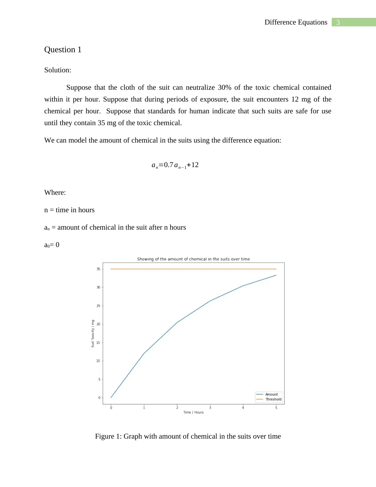
Suppose that the cloth of the suit can neutralize 30% of the toxic chemical contained
within it per hour. Suppose that during periods of exposure, the suit encounters 12 mg of the
chemical per hour. Suppose that standards for human indicate that such suits are safe for use
until they contain 35 mg of the toxic chemical.
We can model the amount of chemical in the suits using the difference equation:
Where:
n = time in hours
an = amount of chemical in the suit after n hours
a0= 0
Figure 1: Graph with amount of chemical in the suits over time
an=0.7 an−1+12

4Difference Equations
According to figure 1 it can be said that up to 5 hours the safety team can work without
having to change their suits. In figure 1 the orange line shows the border or the threshold, up to
which the suits are safe for use, if exceeded then it be harmful for the humans.
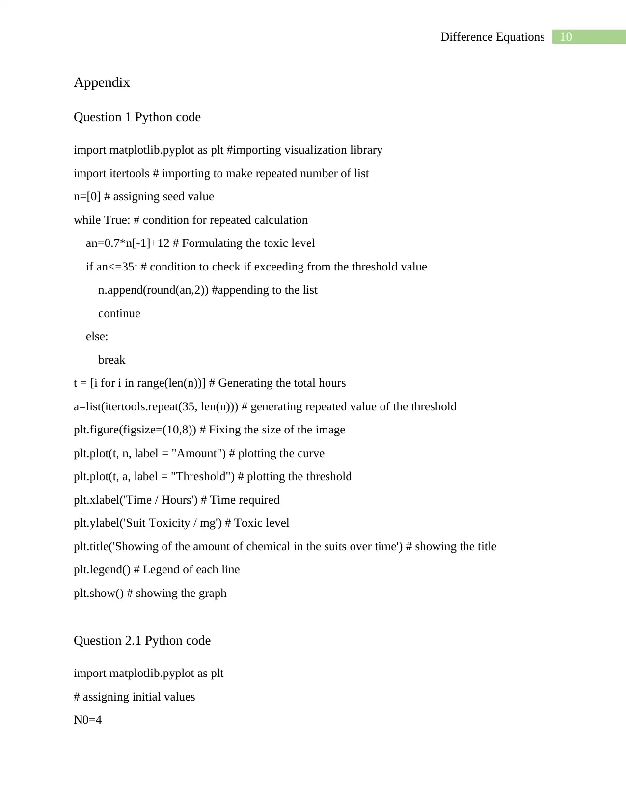
The python code for the same has been attached in the appendix section of the report
which can be run using spyder IDE also proper comments has been added to each line for proper
understanding.
Question 2.1
Solution:
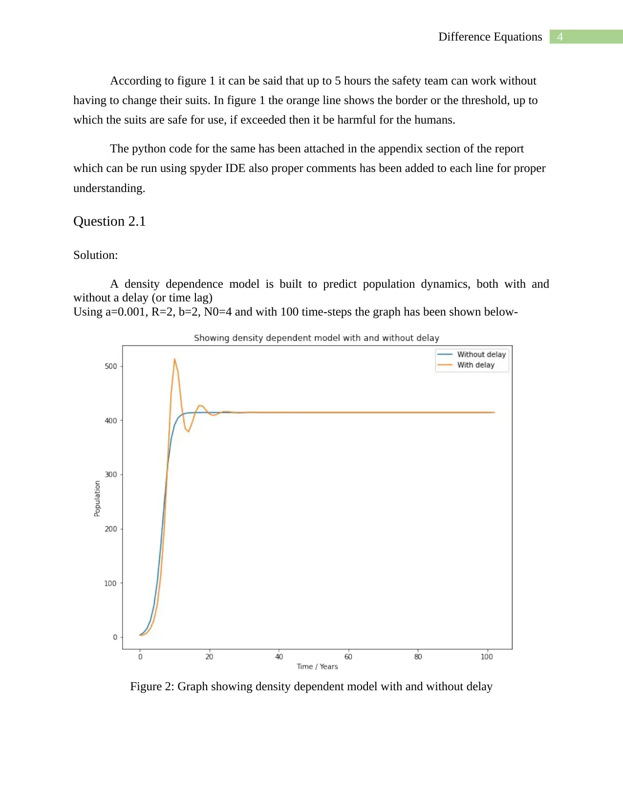
A density dependence model is built to predict population dynamics, both with and
without a delay (or time lag)
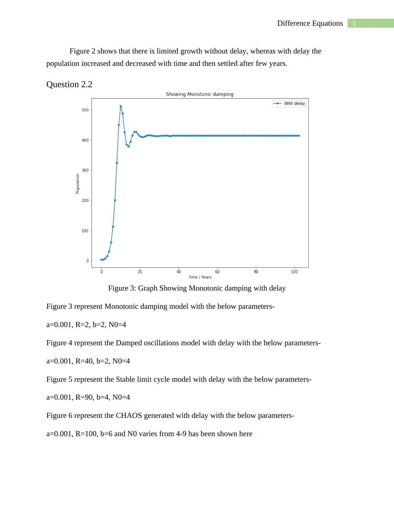
Using a=0.001, R=2, b=2, N0=4 and with 100 time-steps the graph has been shown below-
Figure 2: Graph showing density dependent model with and without delay

5Difference Equations
Figure 2 shows that there is limited growth without delay, whereas with delay the
population increased and decreased with time and then settled after few years.
Question 2.2
Figure 3: Graph Showing Monotonic damping with delay
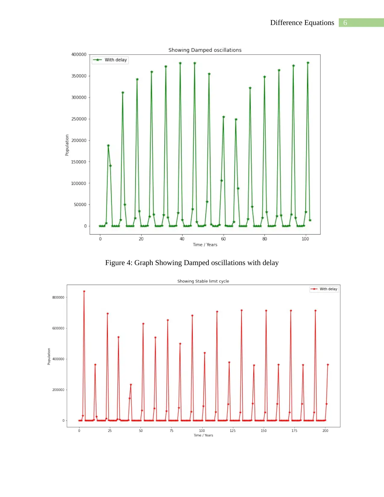
Figure 3 represent Monotonic damping model with the below parameters-
a=0.001, R=2, b=2, N0=4
Figure 4 represent the Damped oscillations model with delay with the below parameters-
a=0.001, R=40, b=2, N0=4
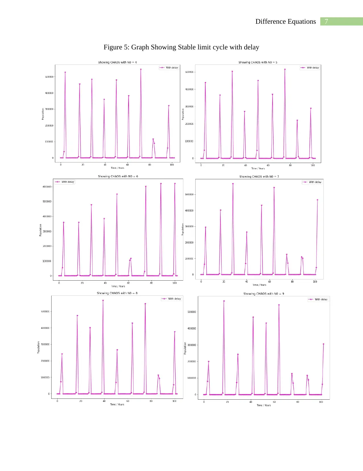
Figure 5 represent the Stable limit cycle model with delay with the below parameters-
a=0.001, R=90, b=4, N0=4
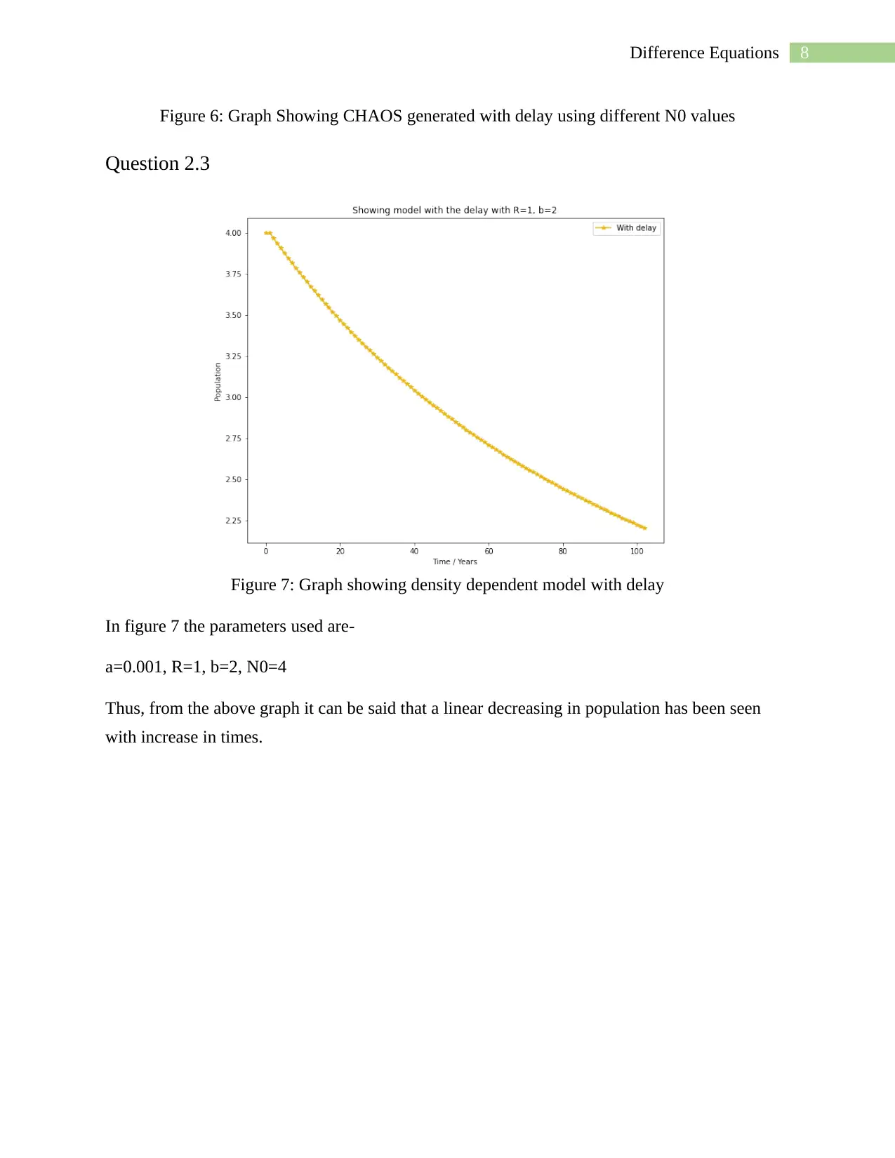
Figure 6 represent the CHAOS generated with delay with the below parameters-
a=0.001, R=100, b=6 and N0 varies from 4-9 has been shown here

6Difference Equations
Figure 4: Graph Showing Damped oscillations with delay

7Difference Equations
Figure 5: Graph Showing Stable limit cycle with delay

8Difference Equations
Figure 6: Graph Showing CHAOS generated with delay using different N0 values
Question 2.3
Figure 7: Graph showing density dependent model with delay
In figure 7 the parameters used are-
a=0.001, R=1, b=2, N0=4
Thus, from the above graph it can be said that a linear decreasing in population has been seen
with increase in times.

9Difference Equations
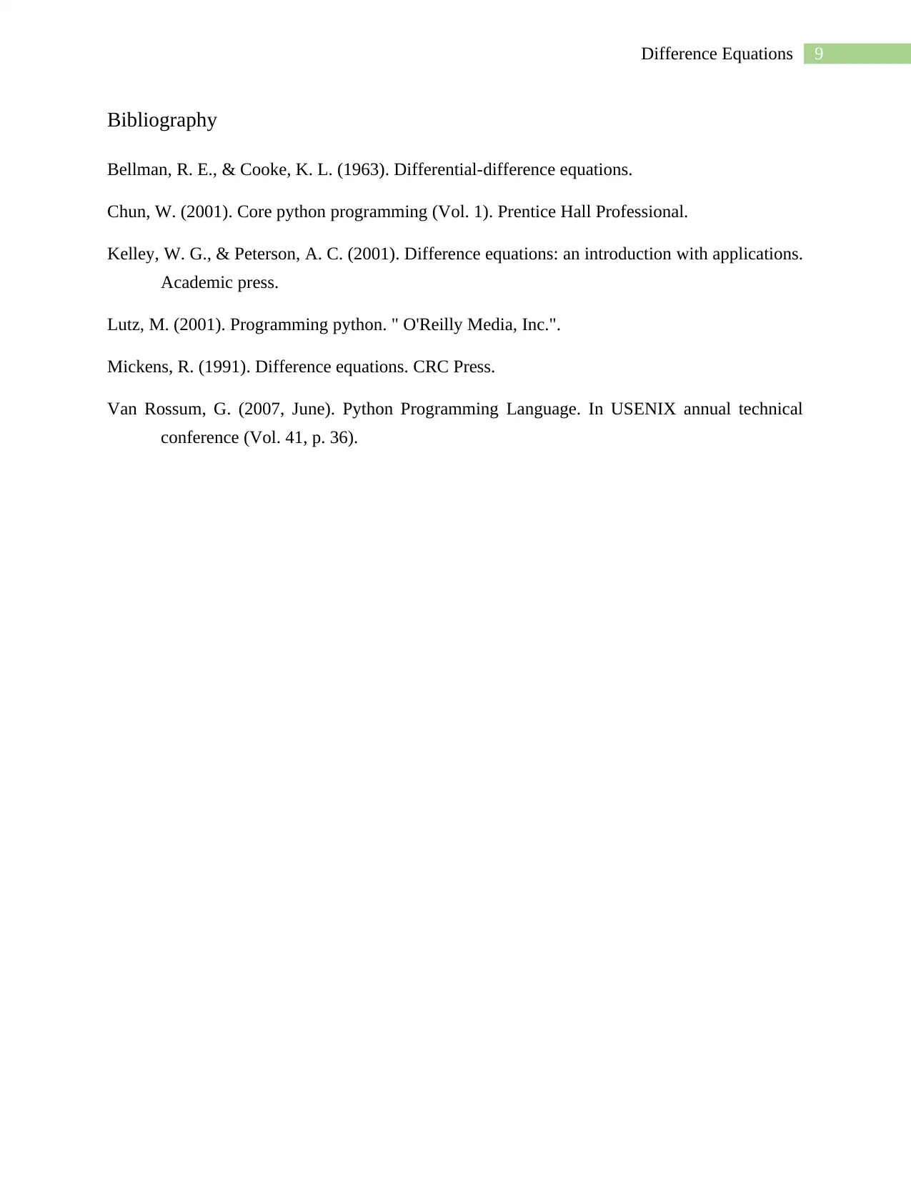
Bibliography
Bellman, R. E., & Cooke, K. L. (1963). Differential-difference equations.
Chun, W. (2001). Core python programming (Vol. 1). Prentice Hall Professional.
Kelley, W. G., & Peterson, A. C. (2001). Difference equations: an introduction with applications.
Academic press.
Lutz, M. (2001). Programming python. " O'Reilly Media, Inc.".
Mickens, R. (1991). Difference equations. CRC Press.
Van Rossum, G. (2007, June). Python Programming Language. In USENIX annual technical
conference (Vol. 41, p. 36).

10Difference Equations
Appendix
Question 1 Python code
import matplotlib.pyplot as plt #importing visualization library
import itertools # importing to make repeated number of list
n=[0] # assigning seed value
while True: # condition for repeated calculation
an=0.7*n[-1]+12 # Formulating the toxic level
if an<=35: # condition to check if exceeding from the threshold value
n.append(round(an,2)) #appending to the list
continue
else:
break
t = [i for i in range(len(n))] # Generating the total hours
a=list(itertools.repeat(35, len(n))) # generating repeated value of the threshold
plt.figure(figsize=(10,8)) # Fixing the size of the image
plt.plot(t, n, label = "Amount") # plotting the curve
plt.plot(t, a, label = "Threshold") # plotting the threshold
plt.xlabel('Time / Hours') # Time required
plt.ylabel('Suit Toxicity / mg') # Toxic level
plt.title('Showing of the amount of chemical in the suits over time') # showing the title
plt.legend() # Legend of each line
plt.show() # showing the graph
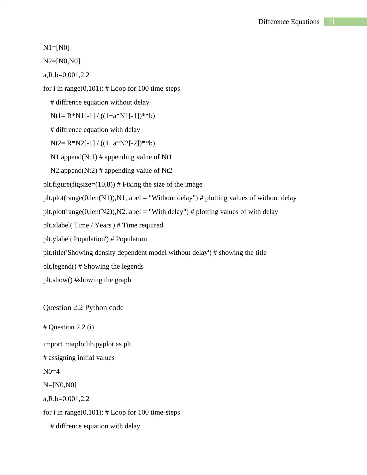
Question 2.1 Python code
import matplotlib.pyplot as plt
# assigning initial values
N0=4

11Difference Equations
N1=[N0]
N2=[N0,N0]
a,R,b=0.001,2,2
for i in range(0,101): # Loop for 100 time-steps
# diffrence equation without delay
Nt1= R*N1[-1] / ((1+a*N1[-1])**b)
# diffrence equation with delay
Nt2= R*N2[-1] / ((1+a*N2[-2])**b)
N1.append(Nt1) # appending value of Nt1
N2.append(Nt2) # appending value of Nt2
plt.figure(figsize=(10,8)) # Fixing the size of the image
plt.plot(range(0,len(N1)),N1,label = "Without delay") # plotting values of without delay
plt.plot(range(0,len(N2)),N2,label = "With delay") # plotting values of with delay
plt.xlabel('Time / Years') # Time required
plt.ylabel('Population') # Population
plt.title('Showing density dependent model without delay') # showing the title
plt.legend() # Showing the legends
plt.show() #showing the graph
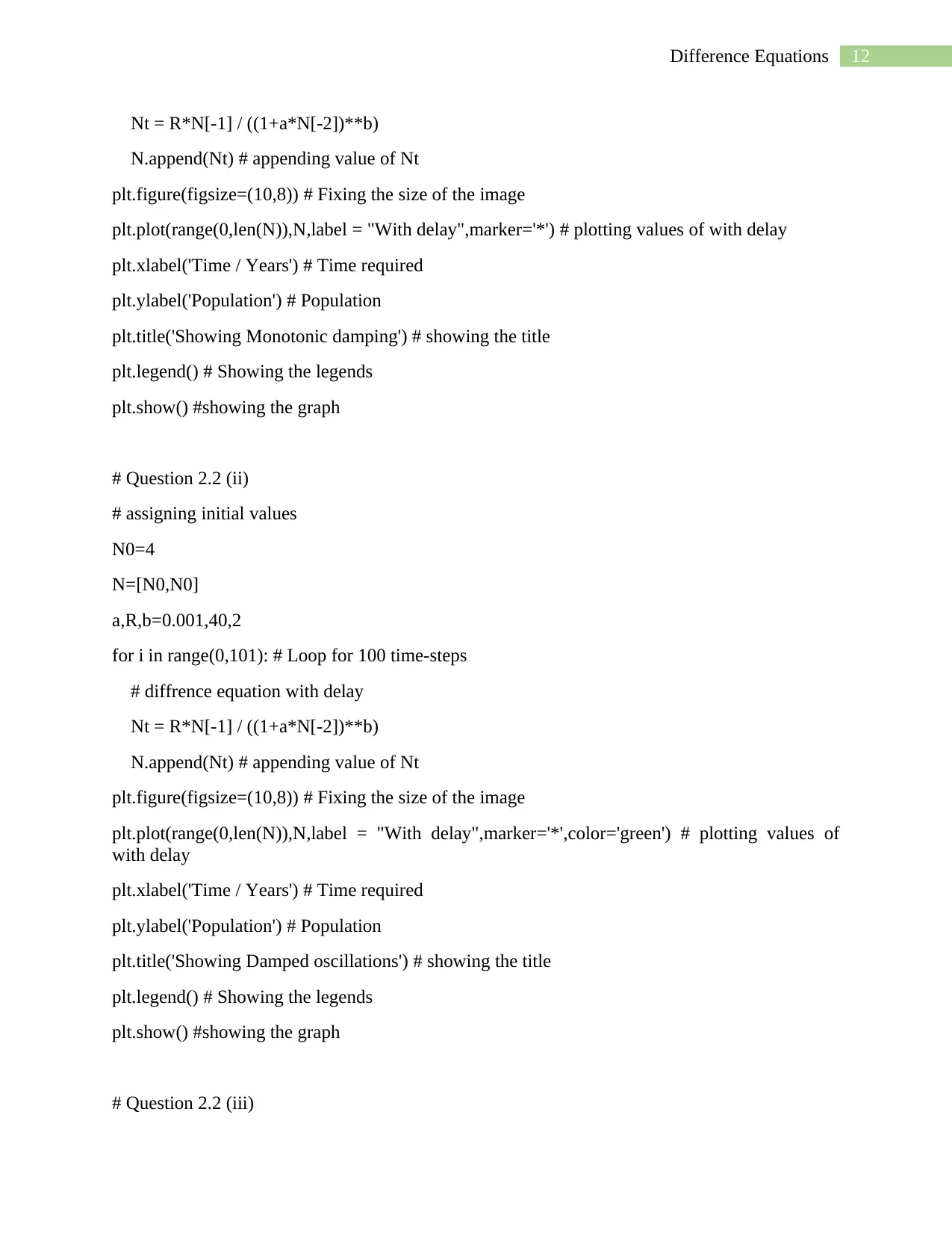
Question 2.2 Python code
# Question 2.2 (i)
import matplotlib.pyplot as plt
# assigning initial values
N0=4
N=[N0,N0]
a,R,b=0.001,2,2
for i in range(0,101): # Loop for 100 time-steps
# diffrence equation with delay

12Difference Equations
Nt = R*N[-1] / ((1+a*N[-2])**b)
N.append(Nt) # appending value of Nt
plt.figure(figsize=(10,8)) # Fixing the size of the image
plt.plot(range(0,len(N)),N,label = "With delay",marker='*') # plotting values of with delay
plt.xlabel('Time / Years') # Time required
plt.ylabel('Population') # Population
plt.title('Showing Monotonic damping') # showing the title
plt.legend() # Showing the legends
plt.show() #showing the graph
# Question 2.2 (ii)
# assigning initial values
N0=4
N=[N0,N0]
a,R,b=0.001,40,2
for i in range(0,101): # Loop for 100 time-steps
# diffrence equation with delay
Nt = R*N[-1] / ((1+a*N[-2])**b)
N.append(Nt) # appending value of Nt
plt.figure(figsize=(10,8)) # Fixing the size of the image
plt.plot(range(0,len(N)),N,label = "With delay",marker='*',color='green') # plotting values of
with delay
plt.xlabel('Time / Years') # Time required
plt.ylabel('Population') # Population
plt.title('Showing Damped oscillations') # showing the title
plt.legend() # Showing the legends
plt.show() #showing the graph
# Question 2.2 (iii)