ELEC376/676 Module 2 Lab Report: Differential Amplifier Investigation

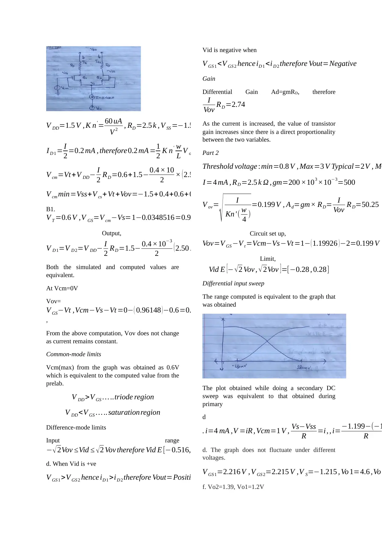
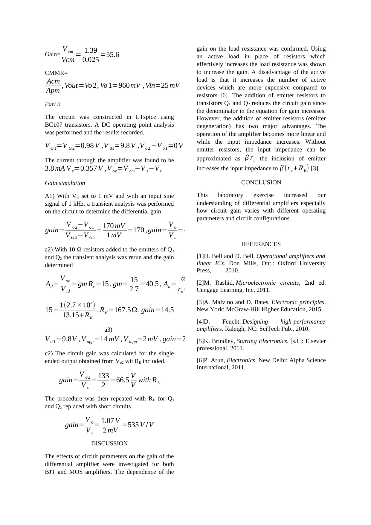
This laboratory report details the investigation of differential amplifiers, focusing on MOSFET and BJT configurations. The report encompasses circuit design, simulation using LTspice, and practical implementation. The study explores the impact of various circuit parameters, such as load resistance and emitter degeneration, on amplifier gain. The report includes pre-lab calculations, circuit setup, gain simulation, and analysis of common-mode and difference-mode limits. The findings reveal the effects of active loads and emitter resistors on circuit performance, providing insights into the trade-offs between gain, linearity, and input impedance. The report also compares simulated and computed values to validate the design and analysis process, providing a comprehensive understanding of differential amplifier behavior.

Laboratory Report
Name
Course
College
Date
Abstract
The effect of variations in circuit parameters were
investigated for both MOS and BJT differential
amplifiers. Increasing the load resistance by using
an active load was shown to increase the gain of
the amplifier. Besides, the use of emitter
degeneration resistances leads to a decrease in the
gain of the amplifier.
INTRODUCTION
Differential amplifiers are amplifiers designed to
amplify a difference of two signals. They limit
noise that is common to both inputs and amplify
the differential signal. This report details the
findings on MOSFET, MOS and BJT differential
amplifiers. This encompasses the design,
simulation and practical implementation of the
three amplifiers. MOSFET are widely used because
of the higher input resistance that is closer to
infinite because the gate pin is not connected to
other pins via a conductor [2]. The first section of
the report details findings of a custom MOSFET
differential pair characteristics. The second section
detail the findings of a simulated and constructed
MOS differential pair made of BS170 circuit pair
and the last section detail simulated and physical
implementation BJT transistor differential
amplifier.
Background to the experimental investigations
Differential amplifiers whether fabricated from
MOSFETs, MOS or BJTs generally require at least
two active devices to operate [4]. A basic
differential amplifier utilizes a single resistors for
the current source as well as for the load. More
complex designs on the contrary may use current
mirror current sources with the load resistors being
replaced by active loads. The use of active loads is
desirable since it increases the output impedance
hence increasing the gain [1]. The optimal
performance of the differential pair requires that
the two input transistors be as closely matched as
possible. In this case, the tail current splits into two
almost equal values which hence the emitter and
collector currents through the transistors will be
almost equal. However, it is impossible to achieve
perfect
matching in practical circuits. Circuit parameters
such as small variations in the base resistors,
collector resistance or a simple mismatch in the Vbe
can produce offset voltages and currents.
There are four different ways of configuring a
differential amplifier. These include differential
input differential output, differential input single
ended output, single ended input differential output
and single ended input single ended output [5].
Small signal analysis
BJT differential amplifier
This analysis assumes that the common mode
voltage is zero and the two transistors are identical
and balanced [2]. Therefore, the input voltages at
the bases will be vid
2 and−vid
2 . The gain of the
amplifier can then be determined from the
differential-mode half circuit as follows.
vod
2 =−gm Rc
vid
2
The differential gain Ad is thus,
Ad = vod
vid
=−gm Rc
MOS differential amplifier
The two equations above also apply for the MOS
differential amplifier with Rc replaced by RD, the
drain resistance.
vod
2 =−gm RD
vid
2 , Ad = vod
vid
=−gm RD
To achieve a higher gm in a MOS circuit, the
biasing current must be higher [2]
Results and circuit designs
Part 1

V DD=1.5 V , K n'=60 uA
V 2 , RD =2.5 k , V SS =−1.5V , W =100um ,V T=0.6V , L=2 um
I D 1 = I
2 =0.2 mA , therefore0.2 mA =1
2 K n' w
L V ov
2 , 2× ( 0.2× 10−3 ) =3V ov
2 ×10−3 , V ov=0.26
V cm=Vt +V DD− I
2 RD =0.6+1.5−0.4 × 10
2 × ( 2.5 ×10−3 ) =1.6 V
V cm min=Vss+V cs + Vt +Vov=−1.5+ 0.4+0.6+ 0.365=−0.135 V ,−0.135V ≤ Vcm ≤1.6 V
B1.
V T =0.6 V ,V GS=V cm−Vs=1−0.0348516=0.965 V , V GS=Vt +Vov ,hence Vov=V GS−Vt =0.965−0.6=0.365V
Output,
V D 1=V D 2=V DD− I
2 RD=1.5− 0.4 ×10−3
2 ( 2.50 .4 ×10−3 )=1 V
Both the simulated and computed values are
equivalent.
At Vcm=0V
Vov=
V GS−Vt ,Vcm−Vs−Vt =0− ( 0.96148 ) −0.6=0.365
,
From the above computation, Vov does not change
as current remains constant.
Common-mode limits
Vcm(max) from the graph was obtained as 0.6V
which is equivalent to the computed value from the
prelab.
V DD >V GS … ..triode region
V DD <V GS … .. saturationregion
Difference-mode limits
Input range
− √ 2Vov ≤Vid ≤ √ 2 Vov therefore Vid E [−0.516,0.516 ]
d. When Vid is +ve
V GS 1 >V GS 2 hence iD 1 >iD 2 therefore Vout=Positive
Vid is negative when
V GS 1 <V GS 2 hence iD 1 <iD 2 therefore Vout=Negative
Gain
Differential Gain Ad=gmRD, therefore
I
Vov RD =2.74
As the current is increased, the value of transistor
gain increases since there is a direct proportionality
between the two variables.
Part 2
Threshold voltage :min=0.8 V , Max=3 V Typical=2V , MO
I =4 mA , RD =2.5 k Ω , gm=200 ×103 ×10−3=500
V ov=
√ I
Kn'( w
4 )
=0.199 V , Ad=gm× RD= I
Vov RD=50.25
Circuit set up,
Vov=V GS −V t =Vcm−Vs−Vt =1− ( 1.19926 ) −2=0.199 V
Limit,
Vid E [− √2 Vov , √2Vov ]=[−0.28 , 0.28]
Differential input sweep
The range computed is equivalent to the graph that
was obtained
The plot obtained while doing a secondary DC
sweep was equivalent to that obtained during
primary
d
. i=4 mA ,V =iR , Vcm=1 V , Vs−Vss
R =i, , i=−1.199−(−1
R
d. The graph does not fluctuate under different
voltages.
V GS 1=2.216 V , V GS 2=2.215 V ,V S=−1.215 , Vo 1=4.6 ,Vo
f. Vo2=1.39, Vo1=1.2V

Gain= V cm
Vcm = 1.39
0.025 =55.6
CMMR=
Acm
Apm , Vout=Vo 2, Vo 1=960mV , Vin=25 mV
Part 3
The circuit was constructed in LTspice using
BC107 transistors. A DC operating point analysis
was performed and the results recorded.
V G 1=V G 2=0.98 V ,V 01=9.8 V ,V o 2 −V o 1=0 V
The current through the amplifier was found to be
3.8 mA V s=0.357 V ,V ov=V cm−V s−V t
Gain simulation
A1) With Vid set to 1 mV and with an input sine
signal of 1 kHz, a transient analysis was performed
on the circuit to determine the differential gain
gain= V o 2−V o 1
V G 2−V G 1
=170 mV
1 mV =170 , gain= V o
V ¿
= 104
1 =104
a2) With 10 Ω resistors added to the emitters of Q1
and Q2 the transient analysis was rerun and the gain
determined
Ad = V od
V id
=gm Rc=15 , gm= 15
2.7 =40.5 , Ad = α Rc
re+ RE
, re=V T
I E
=13.15
15=1(2.7 × 103)
13.15+RE
, RE =167.5Ω, gain=14.5
a3)
V o 1=9.8V , V opp=14 mV , V inpp=2 mV , gain=7
c2) The circuit gain was calculated for the single
ended output obtained from Vo2 wit RE included.
gain=V o 2
V ¿
= 133
2 =66.5 V
V with RE
The procedure was then repeated with RE for Q1
and Q2 replaced with short circuits.
gain=V o
V ¿
= 1.07 V
2 mV =535 V /V
DISCUSSION
The effects of circuit parameters on the gain of the
differential amplifier were investigated for both
BJT and MOS amplifiers. The dependence of the
gain on the load resistance was confirmed. Using
an active load in place of resistors which
effectively increases the load resistance was shown
to increase the gain. A disadvantage of the active
load is that it increases the number of active
devices which are more expensive compared to
resistors [6]. The addition of emitter resistors to
transistors Q1 and Q2 reduces the circuit gain since
the denominator in the equation for gain increases.
However, the addition of emitter resistors (emitter
degeneration) has two major advantages. The
operation of the amplifier becomes more linear and
while the input impedance increases. Without
emitter resistors, the input impedance can be
approximated as β re the inclusion of emitter
increases the input impedance to β (re + RE) [3].
CONCLUSION
This laboratory exercise increased our
understanding of differential amplifiers especially
how circuit gain varies with different operating
parameters and circuit configurations.
REFERENCES
[1]D. Bell and D. Bell, Operational amplifiers and
linear ICs. Don Mills, Ont.: Oxford University
Press, 2010.
[2]M. Rashid, Microelectronic circuits, 2nd ed.
Cengage Learning, Inc, 2011.
[3]A. Malvino and D. Bates, Electronic principles.
New York: McGraw-Hill Higher Education, 2015.
[4]D. Feucht, Designing high-performance
amplifiers. Raleigh, NC: SciTech Pub., 2010.
[5]K. Brindley, Starting Electronics. [s.l.]: Elsevier
professional, 2011.
[6]P. Arun, Electronics. New Delhi: Alpha Science
International, 2011.