Approximation Methods and Solutions of Differential Equations

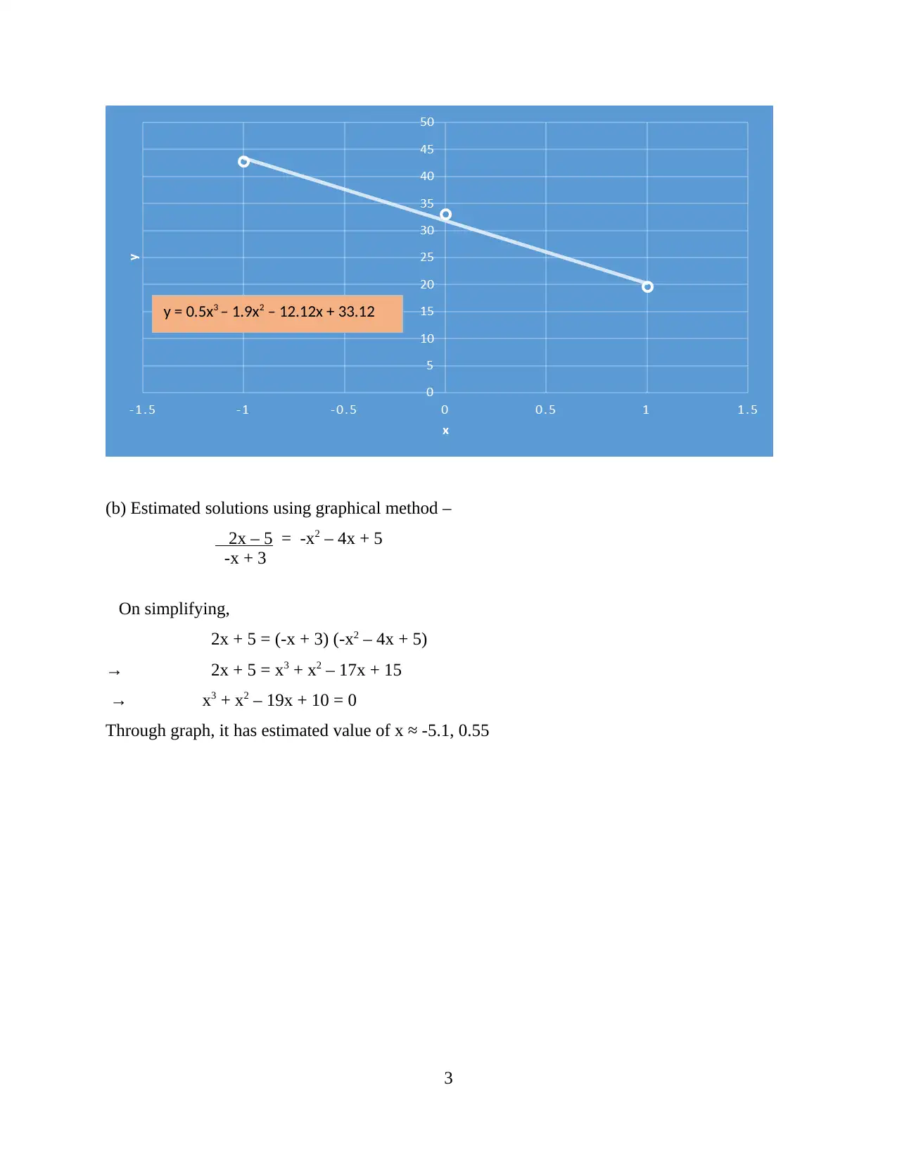
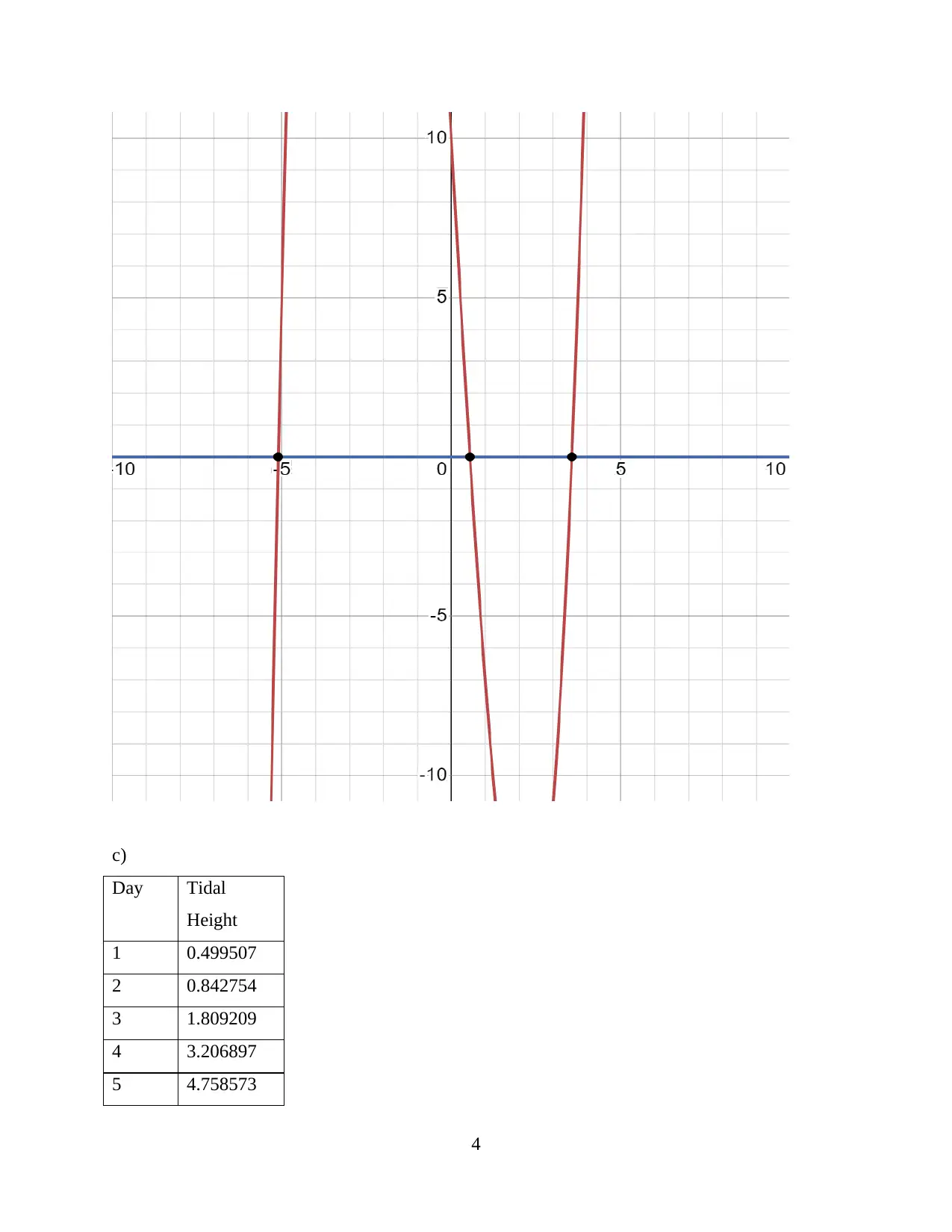
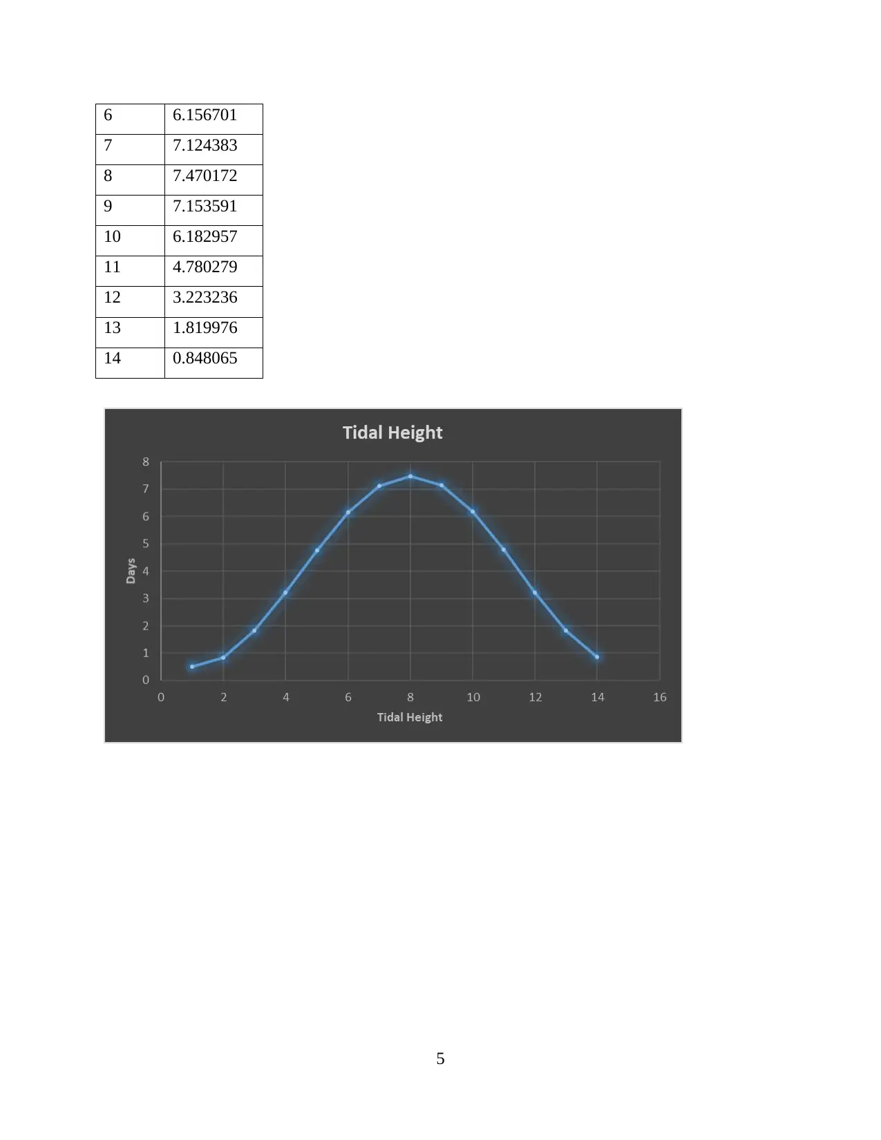
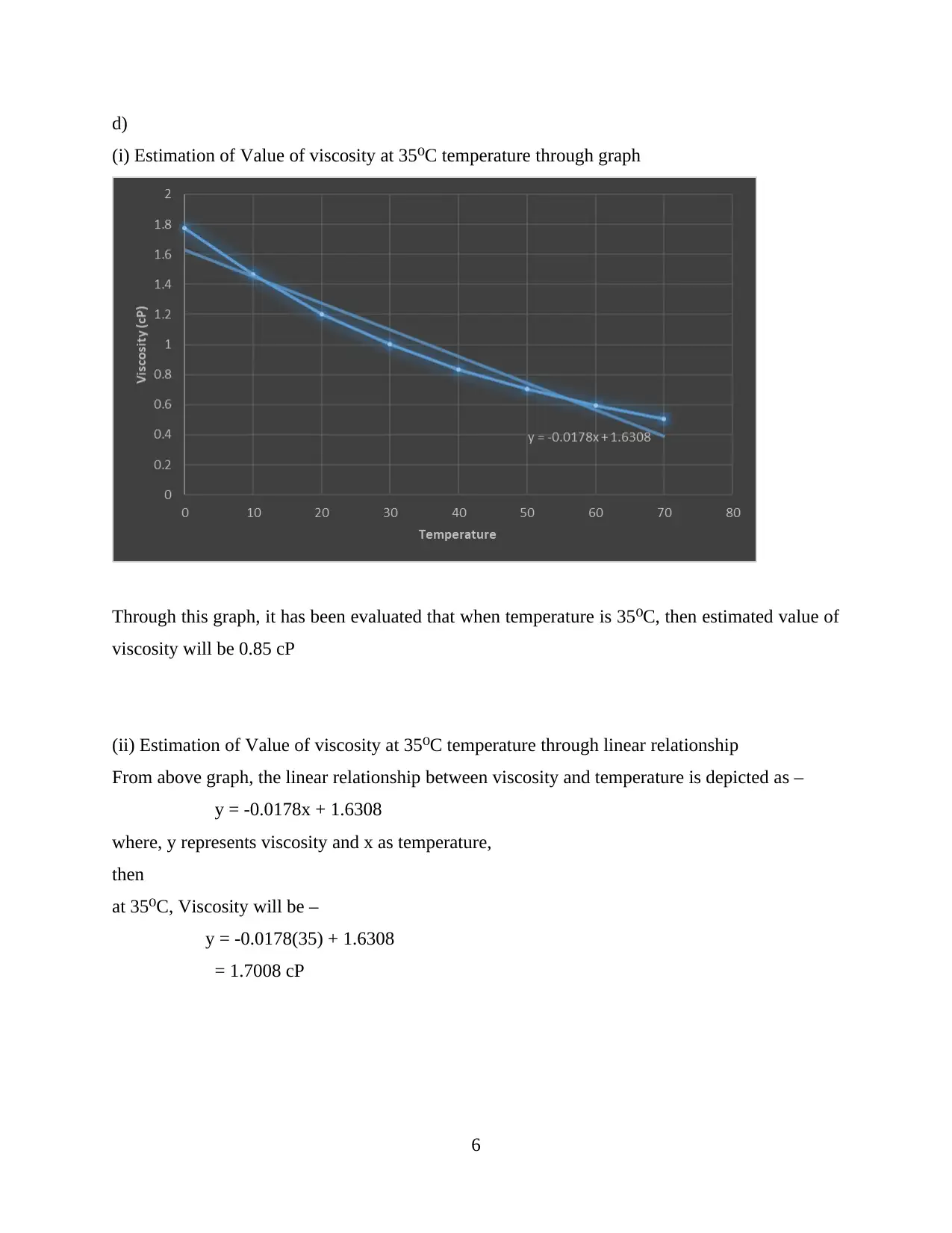
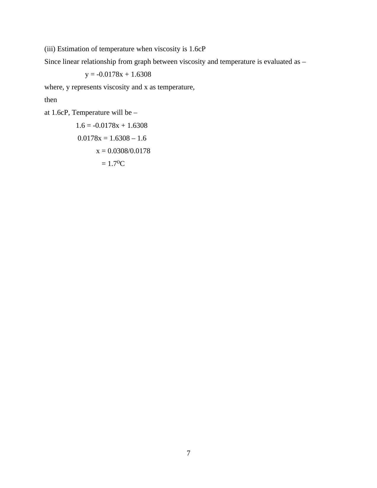
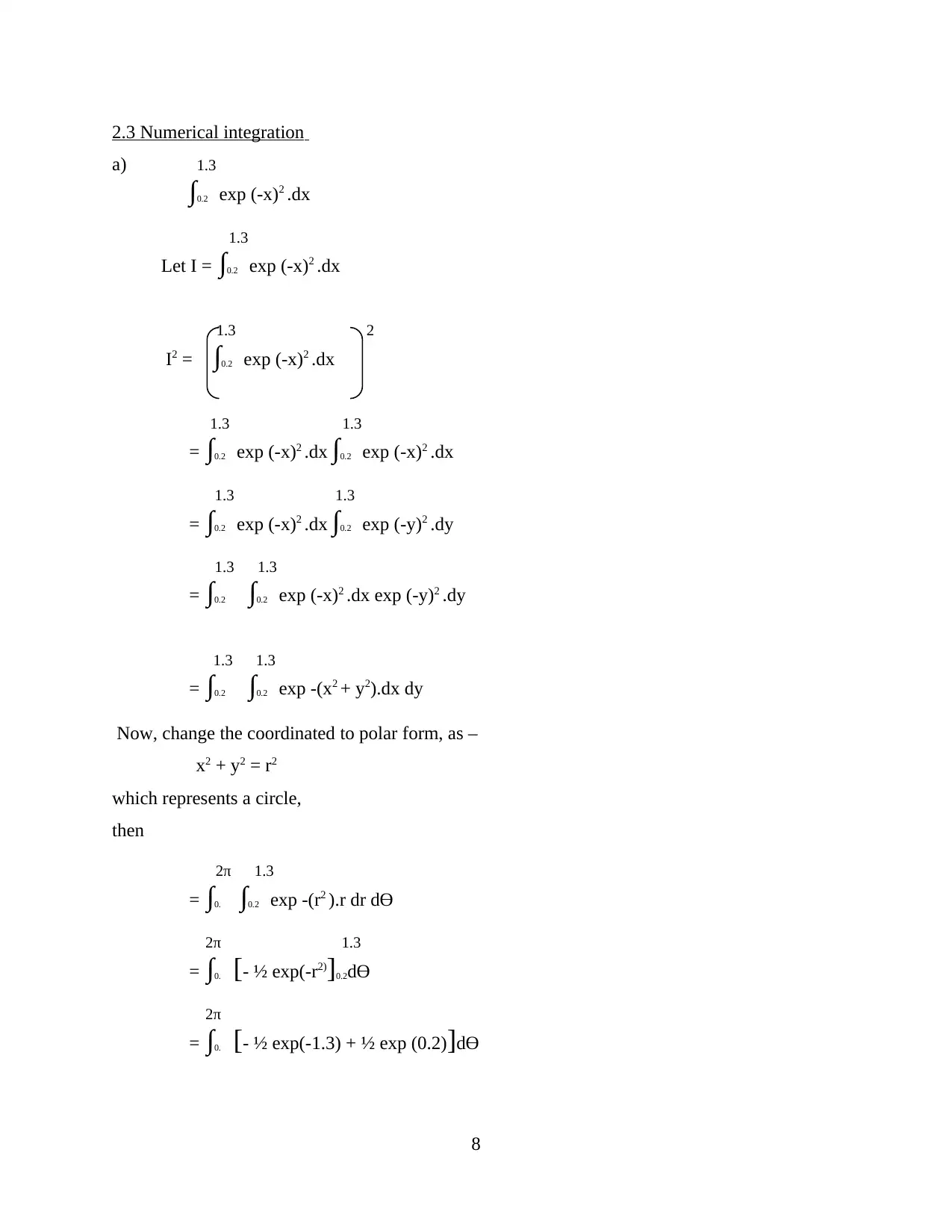
This document presents a comprehensive solution to a differential equations assignment, addressing various problem-solving techniques. The assignment covers sketching graphs, estimating solutions using graphical methods, and analyzing data related to tidal heights and viscosity. It delves into numerical integration, calculating roots through iterative techniques such as Newton's and Regula Falsi methods, and solving differential equations related to damped mechanical systems and electrical circuits. The solutions involve applying concepts of integration, differentiation, and algebraic manipulation to arrive at the solutions. This assignment serves as a valuable resource for students studying calculus and differential equations, offering detailed explanations and step-by-step solutions to enhance understanding and problem-solving skills. The content is designed to aid students in grasping the core principles of differential equations and their practical applications.

Differential equations
approximation methods

Table of Contents
TASK 2............................................................................................................................................1
2.1 & 2.2......................................................................................................................................1
2.3 Numerical integration............................................................................................................8
4.1 (part), 4.2 (part) & 4.5 (part)....................................................................................................12
4.1 (part), 4.2 (part) & 4.5 (part)....................................................................................................13
(b)...............................................................................................................................................13
c)................................................................................................................................................14
4.3 (part), 4.4 & 4.5 (part)..............................................................................................................14
(a)...............................................................................................................................................14
b)................................................................................................................................................16
(c)...............................................................................................................................................16

TASK 2
2.1 & 2.2
(a) Sketch of following graphs -
i) y = 2 – 3 cos (0.5x – π/5)
at x = 100,
y = 2 – 3 cos (50 - π/5)
= 2 – 3 (0.9)
= 2 – 2.7 = -0.7
at x = 200
y = 2 – 3 cos (100 – π/5)
= 2 – 3 (0.4)
= 2 – 1.2 = 0.8
at x = 300
y = 2 – 3 cos (150 – π/5)
= 2 – 3 (-0.4)
= 2 + 1.2 = 3.2
x y
100 -0.7
200 0.8
300 3.2
400 3.8
1

ii) y = 0.5x3 – 1.9x2 – 12.12x + 33.12
at x = 0,
y = 0.5(0)3 – 1.9(0)2 – 12.12(0) + 33.12
= 33.12
at x = 1,
y = 0.5(1)3 – 1.9(1)2 – 12.12(1) + 33.12
= 0.5 – 1.9 – 12.12 + 33.12
= 19.6
at x = -1,
y = 0.5(-1)3 – 1.9(-1)2 – 12.12(-1) + 33.12
= -0.5 – 1.9 + 12.12 + 33.12
= 42.84
x y
0 33.12
1 19.6
-1 42.84
2

(b) Estimated solutions using graphical method –
2x – 5 = -x2 – 4x + 5
-x + 3
On simplifying,
2x + 5 = (-x + 3) (-x2 – 4x + 5)
→ 2x + 5 = x3 + x2 – 17x + 15
→ x3 + x2 – 19x + 10 = 0
Through graph, it has estimated value of x ≈ -5.1, 0.55
3
y = 0.5x3 – 1.9x2 – 12.12x + 33.12

c)
Day Tidal
Height
1 0.499507
2 0.842754
3 1.809209
4 3.206897
5 4.758573
4

6 6.156701
7 7.124383
8 7.470172
9 7.153591
10 6.182957
11 4.780279
12 3.223236
13 1.819976
14 0.848065
5

d)
(i) Estimation of Value of viscosity at 35 C temperature through graph⁰
Through this graph, it has been evaluated that when temperature is 35 C, then estimated value of⁰
viscosity will be 0.85 cP
(ii) Estimation of Value of viscosity at 35 C temperature through linear relationship⁰
From above graph, the linear relationship between viscosity and temperature is depicted as –
y = -0.0178x + 1.6308
where, y represents viscosity and x as temperature,
then
at 35 C, Viscosity will be –⁰
y = -0.0178(35) + 1.6308
= 1.7008 cP
6

(iii) Estimation of temperature when viscosity is 1.6cP
Since linear relationship from graph between viscosity and temperature is evaluated as –
y = -0.0178x + 1.6308
where, y represents viscosity and x as temperature,
then
at 1.6cP, Temperature will be –
1.6 = -0.0178x + 1.6308
0.0178x = 1.6308 – 1.6
x = 0.0308/0.0178
= 1.7 C⁰
7

2.3 Numerical integration
a) 1.3
∫0.2 exp (-x)2 .dx
1.3
Let I = ∫0.2 exp (-x)2 .dx
1.3 2
I2 = ∫0.2 exp (-x)2 .dx
1.3 1.3
= ∫0.2 exp (-x)2 .dx ∫0.2 exp (-x)2 .dx
1.3 1.3
= ∫0.2 exp (-x)2 .dx ∫0.2 exp (-y)2 .dy
1.3 1.3
= ∫0.2 ∫0.2 exp (-x)2 .dx exp (-y)2 .dy
1.3 1.3
= ∫0.2 ∫0.2 exp -(x2 + y2).dx dy
Now, change the coordinated to polar form, as –
x2 + y2 = r2
which represents a circle,
then
2π 1.3
= ∫0. ∫0.2 exp -(r2 ).r dr dϴ
2π 1.3
= ∫0. [- ½ exp(-r2)]0.2dϴ
2π
= ∫0. [- ½ exp(-1.3) + ½ exp (0.2)]dϴ
8

2π
= ∫0. [- ½ exp(-1.3) + ½ exp (0.2)]dϴ
= - ½ [ϴ]02π
I2 = π
I = √π
9