Applications of Differential Equations in Various Disciplines

This assignment delves into the wide-ranging applications of differential equations across various scientific and engineering disciplines. It begins with an introduction to the concept and provides motivating examples to illustrate how real-world problems are mathematically modeled using differential equations, including examples related to pollutant concentration in a tank, the shape of a suspension bridge cable, and the vibration of a shear building. The assignment then explores the connections of differential equations to other areas, including physics (classical mechanics, electrodynamics, general relativity, quantum mechanics), biology (predator-prey equations), and chemistry (rate equations). It further provides detailed applications in specific scenarios such as falling objects, Newton's Law of Cooling, radioactive decay, and carbon dating, with mathematical formulations and solutions for each. The assignment is a comprehensive exploration of the utility of differential equations in modeling and solving a variety of problems.

1
Assignment no #1
Application Of Differential Equation
Name: Nauman Tariq
Roll No: 19011519-088
Section: BSCS-19-IV-A
Course: Differential Equation
Course Code: CS-
Submission Date: 12thjan 2022
Submission To: Dr. Aniqa Zulfiqar
DEPARTMENT OF COMPUTER SCIENCE
UNIVERSITY OF GUJRAT

2
Table of Contents
INTRODUCTION.......................................................................................................................................3
2. MOTIVATING EXAMPLES.....................................................................................................................3
Motivating example-1.............................................................................................................................3
Motivating example-2.............................................................................................................................3
Motivating example-3.............................................................................................................................3
APPLICATIONS AND CONNECTIONS TO OTHER AREAS............................................................................4
3.1 In physics...........................................................................................................................................4
1) Classical mechanics:...........................................................................................................................4
2) Electrodynamics:.................................................................................................................................4
3) General relativity:................................................................................................................................4
4) Quantum mechanics:...........................................................................................................................4
5) Other important equations:................................................................................................................5
3.2 In biology...........................................................................................................................................5
3.3 In chemistry.......................................................................................................................................5
APPLICATION OF DIFFERENTIAL EQUATION IN FALLING OBJECT.............................................................5
APPLICATION OF DIFFERENTIAL EQUATION IN NEWTON’S LAW OF COOLING...................................6
5.3 Radio-active Decay and Carbon Dating..............................................................................................7
5.4 Carbon Dating....................................................................................................................................7
6.CONCLUSION........................................................................................................................................8

3
INTRODUCTION
The Differential equations have wide applications in various engineering and
science disciplines. In general, modeling of the variation of a physical quantity, such as
temperature, pressure, displacement, velocity, stress, strain, current, voltage, or
concentration of a pollutant, with the change of time or location, or both would result in
differential equations. Similarly, studying the variation of some physical quantities on
other physical quantities would also lead to differential equations. In fact, many
engineering subjects, such as mechanical vibration or structural dynamics, heat
transfer, or theory of electric circuits, are founded on the theory of differential
equations. It is practically important for engineers to be able to model physical
problems using mathematical equations, and then solve these equations so that the
behavior of the systems concerned can be studied.
2. MOTIVATING EXAMPLES
It is important for engineers to be able to model physical problems using mathematical
equations, and then solve these equations so that the behavior of the systems
concerned can be studied. In this section, a few examples are presented to illustrate
how practical problems are modeled mathematically and how differential equations
arise in them.
Motivating example-1
A tank contains a liquid of volume V(t), which is polluted with a pollutant concentration
in percentage of c(t) at time t. To reduce the pollutant concentration, an inflow of rate
Qin is injected to the tank. Unfortunately, the inflow is also polluted but to a lesser
degree with a pollutant concentration cin. It is assumed that the inflow is perfectly
mixed with the liquid in the tank instantaneously. An outflow of rate Qout is removed
from the tank. Suppose that, at time t = 0, the volume of the liquid is V0 with a
pollutant concentration of c0.The equation governing the pollutant concentration c(t)
is given by
[V0 + (Qin - Qout)t] (dc(t)/dt)+ Qin c(t) = Qin cin;
With initial condition c(0) = c0. This is a first-order ordinary differential equation
Motivating example-2
Consider the suspension bridge, which consists of the main cable, the hangers, and
the deck. The self-weight of the deck and the loads applied on the deck are
transferred to the cable through the hangers. Set up the Cartesian coordinate system

4
by placing the origin O at the lowest point of the cable. The cable can be modeled as
subjected to a distributed load w(x). The equation governing the shape of the cable is
given by
(d2y/dx2 ) = (w(x)/H)
where H is the tension in the cable at the lowest point O. This is a second-order
ordinary differential equation.
Motivating example-3
Consider the vibration of a single-story shear building under the excitation of
earthquake. The shear building consists of a rigid girder of mass m supported by
columns of combined stiffness k. The vibration of the girder can be described by the
horizontal displacement x(t). The earthquake is modeled by the displacement of the
ground x0(t) as shown. When the girder vibrates, there is a damping force due to the
internal friction between various components of the building, given by
c [x’(t) - x’0(t)]; where c is the damping coefficient.
The relative displacement y(t) = x(t) - x0(t) between the girder and the ground is
governed by the equation
my”(t) + cy’(t) + k y(t) = -mx0”(t), which is a second-order linear ordinary differential
equation.
APPLICATIONS AND CONNECTIONS TO OTHER AREAS
Many fundamental laws of physics and chemistry can be formulated as differential
equations. In biology and economics, differential equations are used to model the
behavior of complex systems. The mathematical theory of differential equations first
developed together with the sciences where the equations had originated and where
the results found application. However, diverse problems, sometimes originating in
quite distinct scientific fields, may give rise to identical differential equations.
Whenever this happens, mathematical theory behind the equations can be viewed
as a unifying principle behind diverse phenomena. As an example, consider
propagation of light and sound in the atmosphere, and of waves on the surface of a
pond. All of them may be described by the same second-order partial differential
equation, the wave equation, which allows us to think of light and sound as forms of
waves, much like familiar waves in the water. Conduction of heat, the theory of which
was developed by Joseph Fourier, is governed by another second-order partial
differential equation, the heat equation. It turns out that many diffusion processes,
while seemingly different, are described by the same equation; the Black-Scholes
equation in finance is, for instance, related to the heat equation.
3.1 In physics
1) Classical mechanics:

5
So long as the force acting on a particle is known, Newton’s second law is sufficient to
describe the motion of a particle. Once independent relations for each force acting
on a particle are available, they can be substituted into Newton’s second law to obtain
an ordinary differential equation, which is called the equation of motion.
2) Electrodynamics:
Maxwell’s equations are a set of partial differential equations that, together with the
Lorentz force law, form the foundation of classical electrodynamics, classical optics,
and electric circuits. These fields in turn underlie modern electrical and
communications technologies. Maxwell’s equations describe how electric and
magnetic fields are generated and altered by each other and by charges and currents.
They are named after the Scottish physicist and mathematician James Clerk Maxwell,
who published an early form of those equations between 1861 and 1862.
3) General relativity:
The Einstein field equations (EFE; also known as ”Einstein’s equations”) are a set of
ten partial differential equations in Albert Einstein’s general theory of relativity which
describe the fundamental interaction of gravitation as a result of space time being
curved by matter and energy. First published by Einstein in 1915 as a tensor
equation, the EFE equate local space time curvature (expressed by the Einstein
tensor) with the local energy and momentum within that space time (expressed by
the stress-energy tensor).
4) Quantum mechanics:
In quantum mechanics, the analogue of Newton’s law is Schrdinger’s equation (a
partial differential equation) for a quantum system (usually atoms, molecules, and
subatomic particles whether free, bound, or localized). It is not a simple algebraic
equation, but in general a linear partial differential equation, describing the time-
evolution of the system’s wave function (also called a ”state function”)
.
5) Other important equations:
Euler-Lagrange equation in classical mechanics, Hamilton’s equations in classical
mechanics, Radioactive decay in nuclear physics, Newton’s law of cooling in
thermodynamics, the wave equation, the heat equation in thermodynamics, Laplace’s
equation, which defines harmonic functions, Poisson’s equation, the geodesic equation,
the Navier-Stokes equations in fluid dynamics, the Diffusion equation in stochastic
processes, the Convection-diffusion equation in fluid dynamics, the Cauchy-Riemann
equations in complex analysis, the Poisson-Boltzmann equation in molecular
dynamics, the shallow water equations, Universal differential equation and the Lorenz
equations whose solutions exhibit chaotic flow.
3.2 In biology
1) Predator-prey equations:

6
The Lotka-Volterra equations, also known as the predator-prey equations, are a pair of
first-order, non-linear, differential equations frequently used to describe the dynamics
of biological systems in which two species interact, one as a predator and the other
as prey.
2) Other important equations
: Verhulst equation - biological population growth, von Bertalanffy model - biological
individual growth, Replicator dynamics - found in theoretical biology and Hodgkin-
Huxley model - neural action potentials.
3.3 In chemistry
Rate equation: The rate law or rate equation for a chemical reaction is a differential
equation that links the reaction rate with concentrations or pressures of reactants and
constant parameters (normally rate coefficients and partial reaction orders). To
determine the rate equation for a particular system one combines the reaction rate with
a mass balance for the system.
3.4 In economics
Important equations: The Black-Scholes Partial Differential Equation, Exogenous growth
model, Malthusian growth model and the Vidale-Wolfe advertising model.
APPLICATION OF DIFFERENTIAL EQUATION IN FALLING OBJECT
An object is dropped from a height at time t = 0. If h(t) is the height of the object at time
t, a(t) the acceleration and v(t) the velocity. The relationships between a, v and h are as
follows:
a(t) = dv/dt; v(t) = dh/dt:
For a falling object, a(t) is constant and is equal to g = -9.8 m/s. Combining the above
differential equations, we can easily deduce the following equation
d2h/dt2 = g
Integrate both sides of the above equation to obtain
dh/dt = gt + v0
Integrate one more time to obtain
h(t) = (1/2)gt2 + v0t +h0
The above equation describes the height of a falling object, from an initial height h0 at
an initial velocity v0, as a function of time.

7
APPLICATION OF DIFFERENTIAL EQUATION IN NEWTON’S LAW
OF COOLING
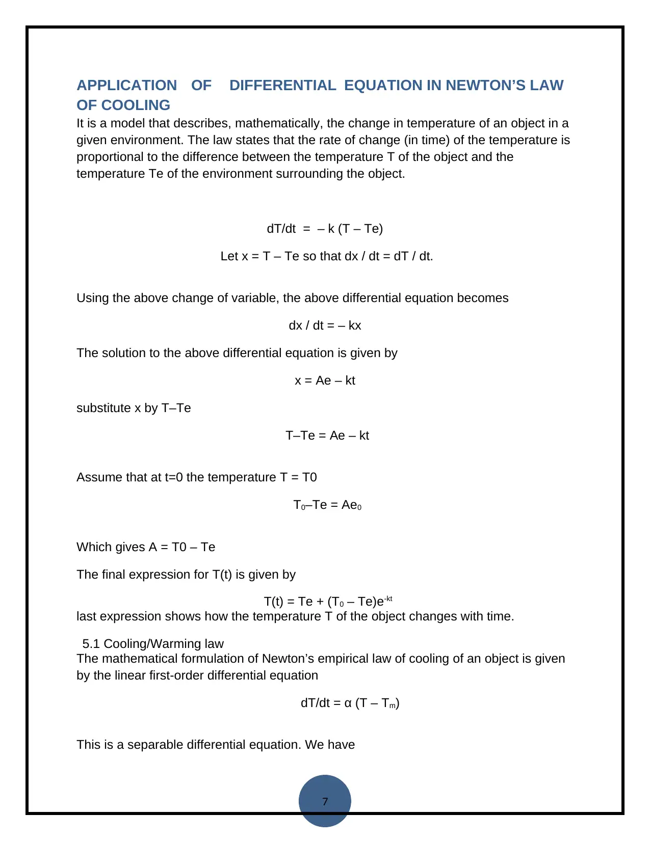
It is a model that describes, mathematically, the change in temperature of an object in a
given environment. The law states that the rate of change (in time) of the temperature is
proportional to the difference between the temperature T of the object and the
temperature Te of the environment surrounding the object.
dT/dt = – k (T – Te)
Let x = T – Te so that dx / dt = dT / dt.
Using the above change of variable, the above differential equation becomes
dx / dt = – kx
The solution to the above differential equation is given by
x = Ae – kt
substitute x by T–Te
T–Te = Ae – kt
Assume that at t=0 the temperature T = T0
T0–Te = Ae0
Which gives A = T0 – Te
The final expression for T(t) is given by
T(t) = Te + (T0 – Te)e-kt
last expression shows how the temperature T of the object changes with time.
5.1 Cooling/Warming law
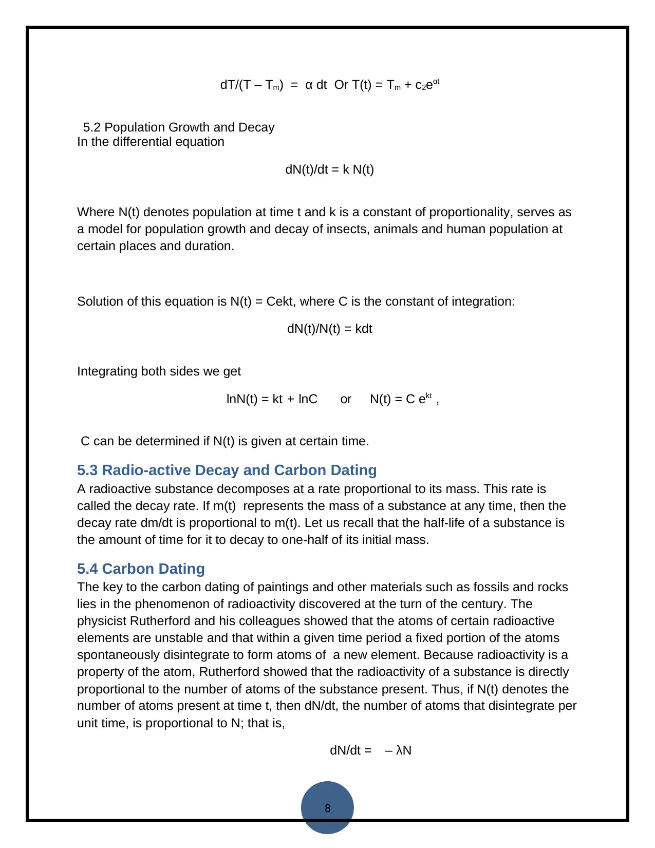
The mathematical formulation of Newton’s empirical law of cooling of an object is given
by the linear first-order differential equation
dT/dt = α (T – Tm)
This is a separable differential equation. We have

8
dT/(T – Tm) = α dt Or T(t) = Tm + c2eαt
5.2 Population Growth and Decay
In the differential equation
dN(t)/dt = k N(t)
Where N(t) denotes population at time t and k is a constant of proportionality, serves as
a model for population growth and decay of insects, animals and human population at
certain places and duration.
Solution of this equation is N(t) = Cekt, where C is the constant of integration:
dN(t)/N(t) = kdt
Integrating both sides we get
lnN(t) = kt + lnC or N(t) = C ekt ,
C can be determined if N(t) is given at certain time.
5.3 Radio-active Decay and Carbon Dating
A radioactive substance decomposes at a rate proportional to its mass. This rate is
called the decay rate. If m(t) represents the mass of a substance at any time, then the
decay rate dm/dt is proportional to m(t). Let us recall that the half-life of a substance is
the amount of time for it to decay to one-half of its initial mass.
5.4 Carbon Dating
The key to the carbon dating of paintings and other materials such as fossils and rocks
lies in the phenomenon of radioactivity discovered at the turn of the century. The
physicist Rutherford and his colleagues showed that the atoms of certain radioactive
elements are unstable and that within a given time period a fixed portion of the atoms
spontaneously disintegrate to form atoms of a new element. Because radioactivity is a
property of the atom, Rutherford showed that the radioactivity of a substance is directly
proportional to the number of atoms of the substance present. Thus, if N(t) denotes the
number of atoms present at time t, then dN/dt, the number of atoms that disintegrate per
unit time, is proportional to N; that is,
dN/dt = – λN

9
5.5 Drug Distribution (Concentration) in Human Body:
To combat the infection to human a body appropriate dose of medicine is essential.
Because the amount of the drug in the human body decreases with time medicine must
be given in multiple doses. The rate at which the level y of the drug in a patient’s blood
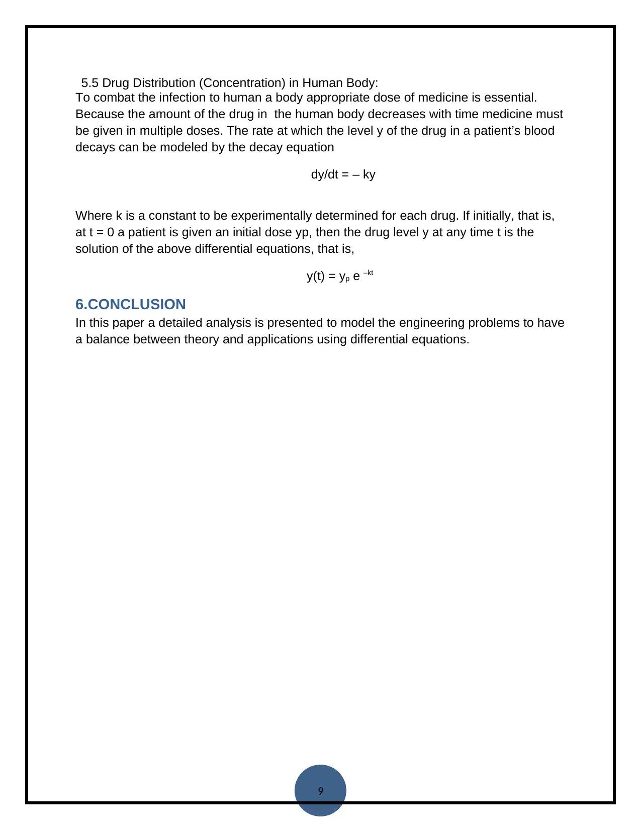
decays can be modeled by the decay equation
dy/dt = – ky
Where k is a constant to be experimentally determined for each drug. If initially, that is,
at t = 0 a patient is given an initial dose yp, then the drug level y at any time t is the
solution of the above differential equations, that is,
y(t) = yp e –kt
6.CONCLUSION
In this paper a detailed analysis is presented to model the engineering problems to have
a balance between theory and applications using differential equations.