Engt5111: Signal Analysis and Video Compression Technical Report
VerifiedAdded on 2022/01/04
|16
|3008
|17
Report
AI Summary
This technical report, prepared for Engt5111, explores digital signal processing concepts. Part I focuses on filter design and signal analysis, including the use of IIR filters for ECG signal processing and MATLAB implementation. It also covers spectrogram analysis, detailing its types, working principles, and applications. The report analyzes a 'couch playing' WAV file using MATLAB to illustrate signal analysis in time and frequency domains. Part II delves into video processing, specifically the merits of the BD method over other codecs. The report includes a discussion of video quality evaluation and provides MATLAB code for implementing the BD test to determine average differences. The report concludes with a comprehensive list of references.
Digital signal processing
Technical report
Engt5111 2018-19
Signal Analysis and Video Compression
Student Name
Student ID Number
Institutional Affiliation
Location
Date of Submission
Technical report
Engt5111 2018-19
Signal Analysis and Video Compression
Student Name
Student ID Number
Institutional Affiliation
Location
Date of Submission
Paraphrase This Document
Need a fresh take? Get an instant paraphrase of this document with our AI Paraphraser
PART I (FILTER DESIGN & SIGNAL ANALYSIS)
PROBLEM 1
Question 1
An ECG is corrupted by muscle noise. The use of this filter to process the signal is quite
necessary as it eliminates the high frequency harmonics which are brought about by measuring
the muscle movements. The ECG signal is measured on the skin using the sensors. The filter is
obtained using the input-output difference equation given as,
y [ n ] = 1
21 (−2 x [ n ] +3 x [ n−1 ]+ 6 x [ n−2 ] +7 x [n−3 ] +3 x [ n−5 ]−2 x [ n−6 ] )
Question 2
Recursive filter design for the ECG signal above,
Digital filter are used to remove frequencies in the low band, high band or a section band from a
digital signal which may be converted from continuous time function to an output function. The
recursive filter repeats itself by using the past output values for the computation of the current
output, such that,
past output vales ( y [ n−i ] )
current values y [ n ]
For instance,
y [ n ] = 1
21 (−2 x [ n ] +3 x [ n−1 ]+ 6 x [ n−2 ] +7 x [n−3 ] +3 x [ n−5 ]−2 x [ n−6 ] )
The generalized difference equation for the linear time invariant system, considering it to be a
causal system,
∑
k=0
N
a [ k ] y [ n−k ]=∑
k=0
M
b [ k ] x [n−k ]
When the value of a[0] is unity, the equation is given as,
1
y [ n ] =∑
k=0
M
b [ k ] x [ n−k ]−∑
k=0
N
a [ k ] y [ n−k ]
To obtain the frequency response of the system,
H ( Ω )=
∑
k=0
M
b [ k ] e−ik Ω
e0 +∑
k=1
N
a [ k ] e−ikΩ
=
∑
k=0
M
b [ k ] e−ik Ω
1+∑
k=1
N
a [ k ] e−ik Ω
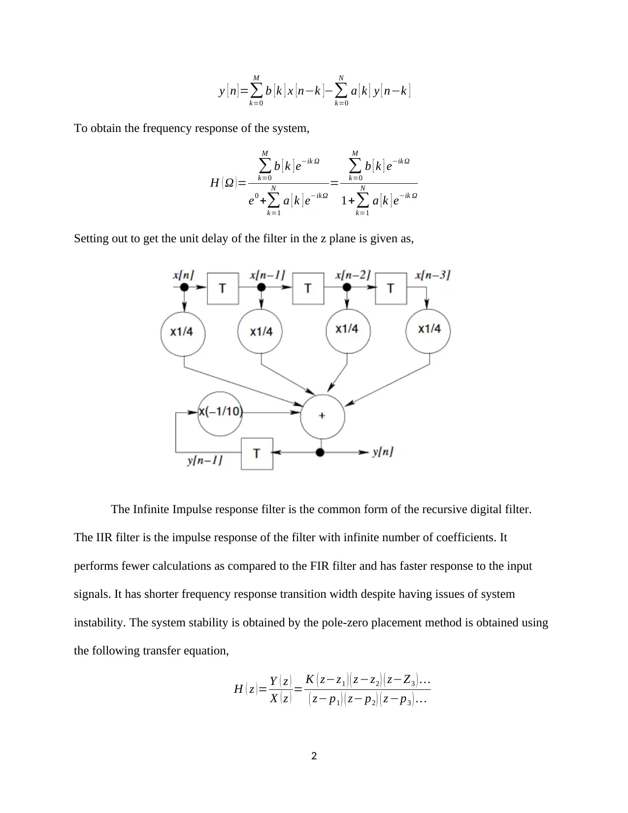
Setting out to get the unit delay of the filter in the z plane is given as,
The Infinite Impulse response filter is the common form of the recursive digital filter.
The IIR filter is the impulse response of the filter with infinite number of coefficients. It
performs fewer calculations as compared to the FIR filter and has faster response to the input
signals. It has shorter frequency response transition width despite having issues of system
instability. The system stability is obtained by the pole-zero placement method is obtained using
the following transfer equation,
H ( z ) = Y ( z )
X ( z ) = K ( z−z1 ) ( z −z2 ) ( z−Z3 ) …
( z− p1 ) ( z− p2 ) ( z −p3 ) …
2
k=0
M
b [ k ] x [ n−k ]−∑
k=0
N
a [ k ] y [ n−k ]
To obtain the frequency response of the system,
H ( Ω )=
∑
k=0
M
b [ k ] e−ik Ω
e0 +∑
k=1
N
a [ k ] e−ikΩ
=
∑
k=0
M
b [ k ] e−ik Ω
1+∑
k=1
N
a [ k ] e−ik Ω
Setting out to get the unit delay of the filter in the z plane is given as,
The Infinite Impulse response filter is the common form of the recursive digital filter.
The IIR filter is the impulse response of the filter with infinite number of coefficients. It
performs fewer calculations as compared to the FIR filter and has faster response to the input
signals. It has shorter frequency response transition width despite having issues of system
instability. The system stability is obtained by the pole-zero placement method is obtained using
the following transfer equation,
H ( z ) = Y ( z )
X ( z ) = K ( z−z1 ) ( z −z2 ) ( z−Z3 ) …
( z− p1 ) ( z− p2 ) ( z −p3 ) …
2
⊘ This is a preview!⊘
Do you want full access?
Subscribe today to unlock all pages.
Trusted by 1+ million students worldwide
Question 3
Using MATLAB to implement the filter designed using the IIR filter, using the input signal,
x [ n ]=cos ( 0.35 n )
sfs = 98.5;
fcuts = [0.5 1.0 45 46];
mags = [0 1 0];
devs = [0.05 0.01 0.05];
[n,Wn,beta,ftype] = kaiserord(fcuts,mags,devs,sfs);
n = n + rem(n,2);
hh = fir1(n,Wn,ftype,kaiser(n+1,beta),'scale');
figure(1)
freqz(hh, 1, 2^14, sfs)
PROBLEM 2
Spectrogram of a signal
A spectrogram is a visual way of symbolizing the magnitude of a signal or sound over
time at diverse frequencies existing in a certain waveform. Occasionally know as voiceprints,
sonographs or voice graphs. Spectrograms are normally used to show frequencies of sound
waves generated by a person, animal or even a gadget as recorded. Spectrograms are extremely
comprehensive, error free representation of audios displayed either in 2D or 3D. An audio is
displayed on a graph depending on time and frequency, with radiance or highness showing
magnitude. A spectrogram displays changes for each and every frequency element in a signal. In
a graph, the vertical axis represents the frequency whereas the horizontal axis represents time.
Types of Spectrogram
3
Paraphrase This Document
Need a fresh take? Get an instant paraphrase of this document with our AI Paraphraser
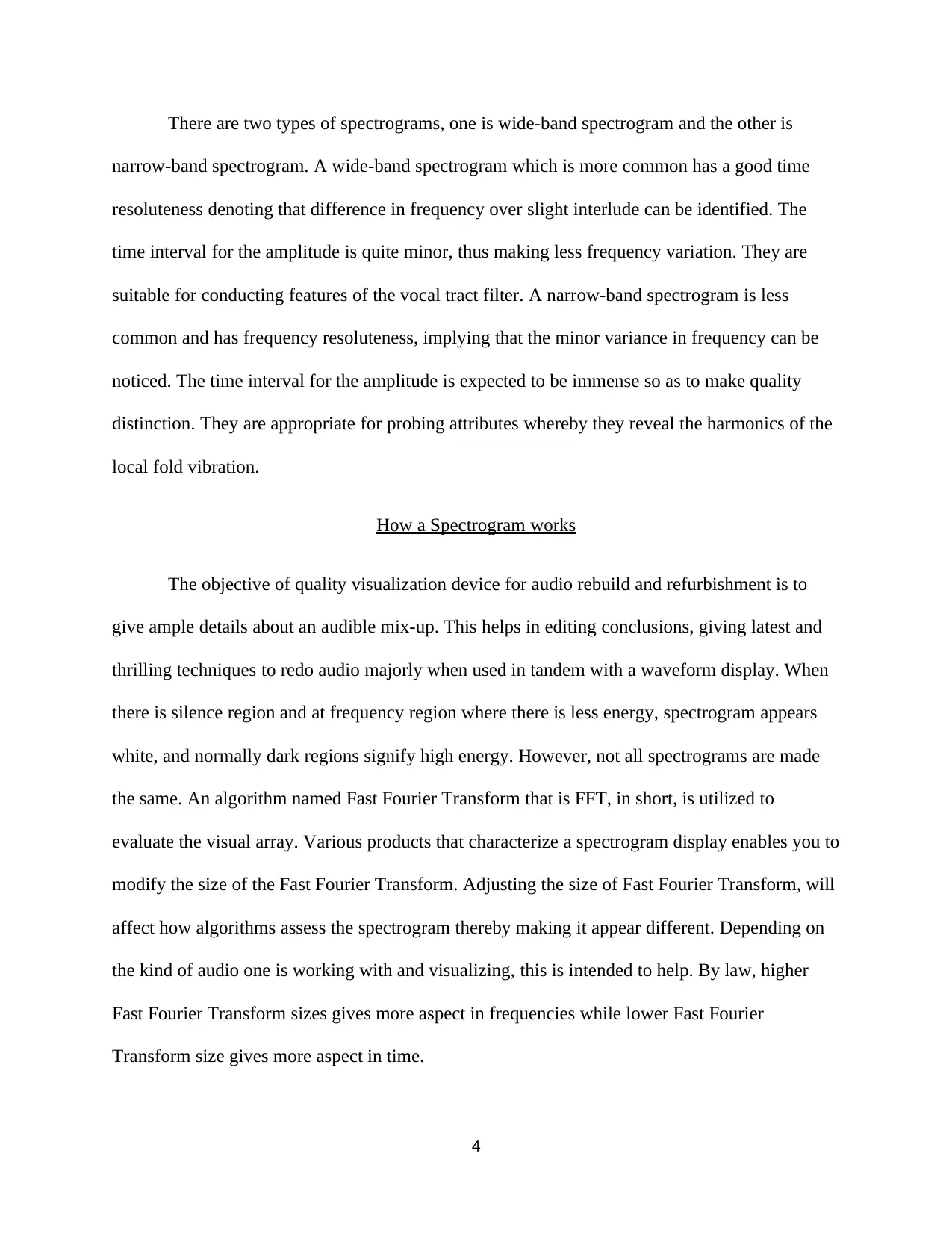
There are two types of spectrograms, one is wide-band spectrogram and the other is
narrow-band spectrogram. A wide-band spectrogram which is more common has a good time
resoluteness denoting that difference in frequency over slight interlude can be identified. The
time interval for the amplitude is quite minor, thus making less frequency variation. They are
suitable for conducting features of the vocal tract filter. A narrow-band spectrogram is less
common and has frequency resoluteness, implying that the minor variance in frequency can be
noticed. The time interval for the amplitude is expected to be immense so as to make quality
distinction. They are appropriate for probing attributes whereby they reveal the harmonics of the
local fold vibration.
How a Spectrogram works
The objective of quality visualization device for audio rebuild and refurbishment is to
give ample details about an audible mix-up. This helps in editing conclusions, giving latest and
thrilling techniques to redo audio majorly when used in tandem with a waveform display. When
there is silence region and at frequency region where there is less energy, spectrogram appears
white, and normally dark regions signify high energy. However, not all spectrograms are made
the same. An algorithm named Fast Fourier Transform that is FFT, in short, is utilized to
evaluate the visual array. Various products that characterize a spectrogram display enables you to
modify the size of the Fast Fourier Transform. Adjusting the size of Fast Fourier Transform, will
affect how algorithms assess the spectrogram thereby making it appear different. Depending on
the kind of audio one is working with and visualizing, this is intended to help. By law, higher
Fast Fourier Transform sizes gives more aspect in frequencies while lower Fast Fourier
Transform size gives more aspect in time.
4

Spectrogram Reading
Verbal expression entails quavering resulting from the vocal tract. Vibrations can be
signified by the waveforms resulting from talking. A spectrogram can be decoded when a
waveform is examined into its frequency elements. The range at which a person’s audio speech
ranges is between 20Hz and 20 kHz. A person is not in a position to hear trembles which
transpire at a frequency less than 20 counts in a neither second nor frequency higher than 20
kHz. Sounds resulting from talking have power at all frequencies in the clear scope. Human
speech and musical signals are key sources of input in signal processing and analysis such that
they provide a good avenue for the determination of the signal information.
Fourier analysis is a mathematical mastery applied in the speech waveform so as to
unearth what frequencies are existing whenever there is a signal resulting from speaking. A
spectrum is the outcome of Fourier analysis. Adjacent spectra normally differ gradually and
evenly, showing gradual motion of the vocal tract in relation to the stretch of analysis window. A
waveform and a spectrogram are shown by a similar portion of speech one on top of the other.
Such arrangement makes it easy to compare formats in waveform and those in the spectrogram.
Applications of Spectrogram
Spectrograms are massively used in areas of sonar, music, speech and radar processing
among others. It is used to single out words that are spoken phonetically and to examine calls of
animals. It can be triggered by an optical spectrometer, a bank of band-pass filters or Fourier
transform. It is also interesting that some images can be hidden in music and can only be viewed
by using a spectrogram of the suitable section of the audio. They are also used to show dispersed
frameworks quantified with vector network analyzers. Spectrograms can used to perceive when
5
⊘ This is a preview!⊘
Do you want full access?
Subscribe today to unlock all pages.
Trusted by 1+ million students worldwide
someone is talking through the recurrent neural networks. Also, spectrograms are helpful in
aiding in overpowering speech shortfalls and also in speech coaching to the deaf. Spectrogram is
used to study frequency modulation in animal calls.
There are many software used in the determination of a signal spectrogram. Some of
these signal processing software are Octave for Raspberry Pi, Matlab R2018b, SimScape
software, etc. As a result, it is possible to obtain the signal in the analog form save it in digital
form while preparing it for processing. The spectrogram is a representation of the signal based on
the regions. There are darker regions that demonstrate the signal power as a result of speech or
musical impact while some white and blue areas demonstrate the lower powered sections. The
signal can be analyzed in sections to determine the power at a given point of the speech and as a
result information about the signal can be deduced. For instance, the wav file analyzed in the
next question is a relevant example demonstrating the proper signal analysis of the system. The
signal, therefore, is given such that the spectrogram has both the power and the frequency
components and the signal attributes. The common plot function is based on the time domain
while the spectrogram represents the signal in the frequency domain and demonstrates the signal
power.
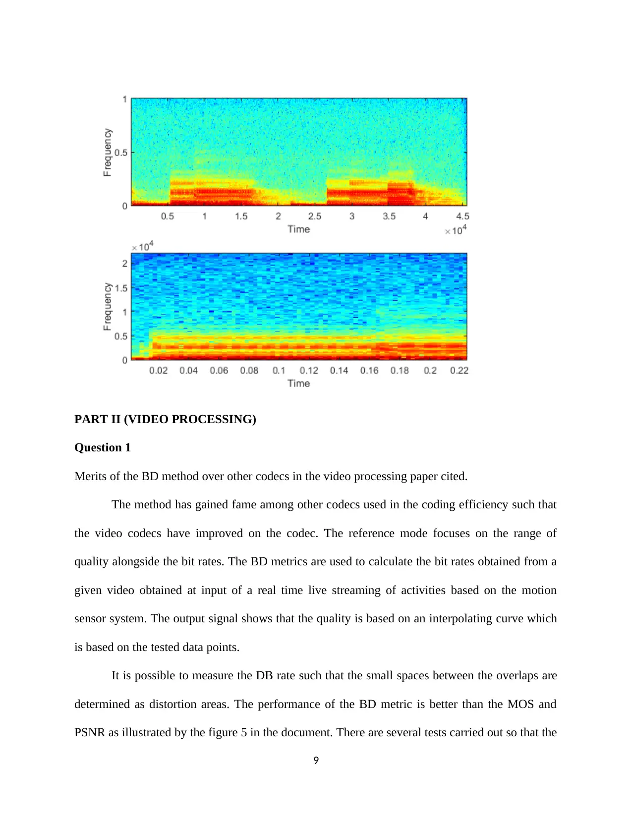
Question 2
Analyzing the couch playing wav file as attached in the zip file, the following functions were
used to determine the signal spectrogram as well as play the sound from the digital file form.
%PART I
%problem 2
[y,fs]=audioread('couchplayin.wav');
sound(y,fs);
6
aiding in overpowering speech shortfalls and also in speech coaching to the deaf. Spectrogram is
used to study frequency modulation in animal calls.
There are many software used in the determination of a signal spectrogram. Some of
these signal processing software are Octave for Raspberry Pi, Matlab R2018b, SimScape
software, etc. As a result, it is possible to obtain the signal in the analog form save it in digital
form while preparing it for processing. The spectrogram is a representation of the signal based on
the regions. There are darker regions that demonstrate the signal power as a result of speech or
musical impact while some white and blue areas demonstrate the lower powered sections. The
signal can be analyzed in sections to determine the power at a given point of the speech and as a
result information about the signal can be deduced. For instance, the wav file analyzed in the
next question is a relevant example demonstrating the proper signal analysis of the system. The
signal, therefore, is given such that the spectrogram has both the power and the frequency
components and the signal attributes. The common plot function is based on the time domain
while the spectrogram represents the signal in the frequency domain and demonstrates the signal
power.
Question 2
Analyzing the couch playing wav file as attached in the zip file, the following functions were
used to determine the signal spectrogram as well as play the sound from the digital file form.
%PART I
%problem 2
[y,fs]=audioread('couchplayin.wav');
sound(y,fs);
6
Paraphrase This Document
Need a fresh take? Get an instant paraphrase of this document with our AI Paraphraser
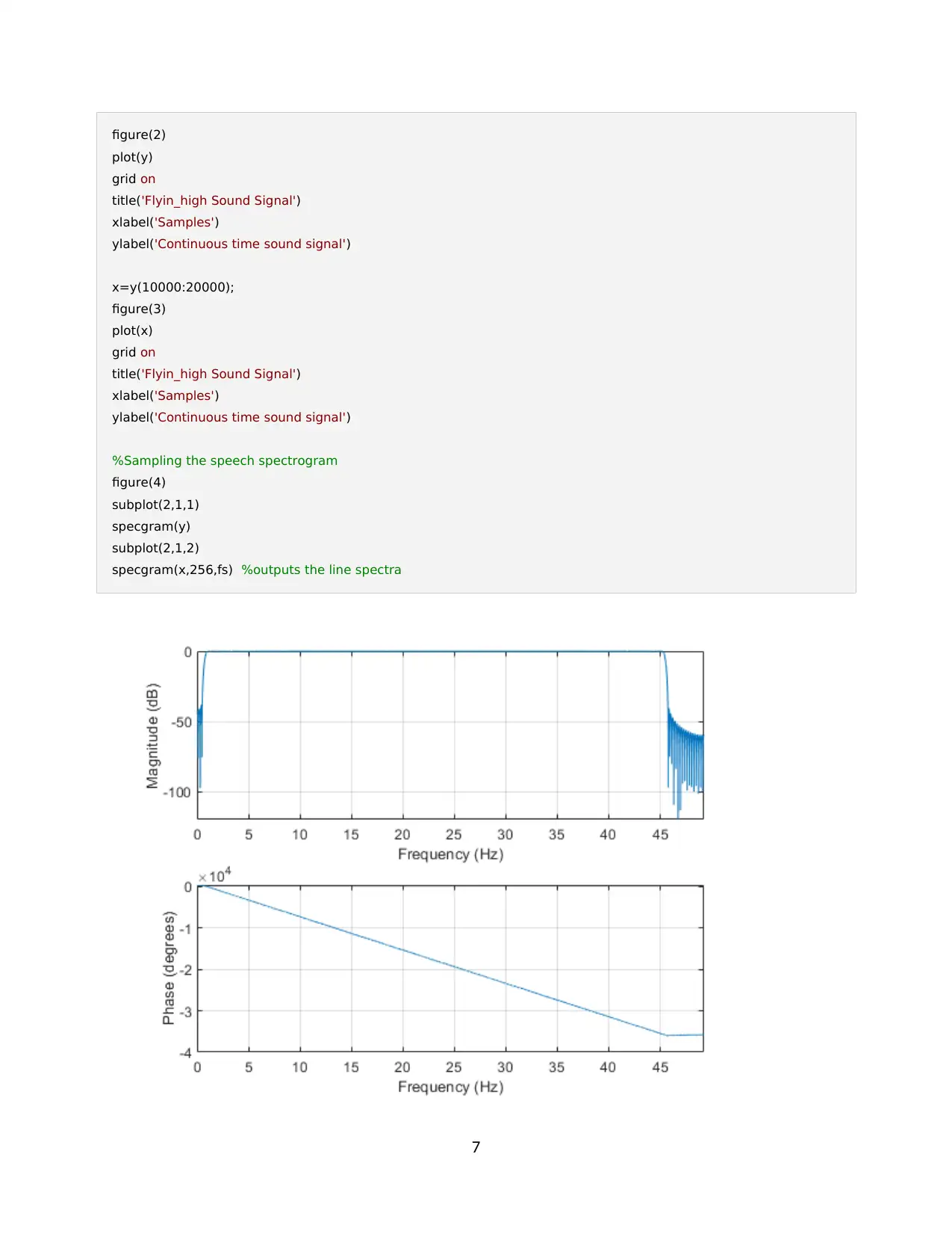
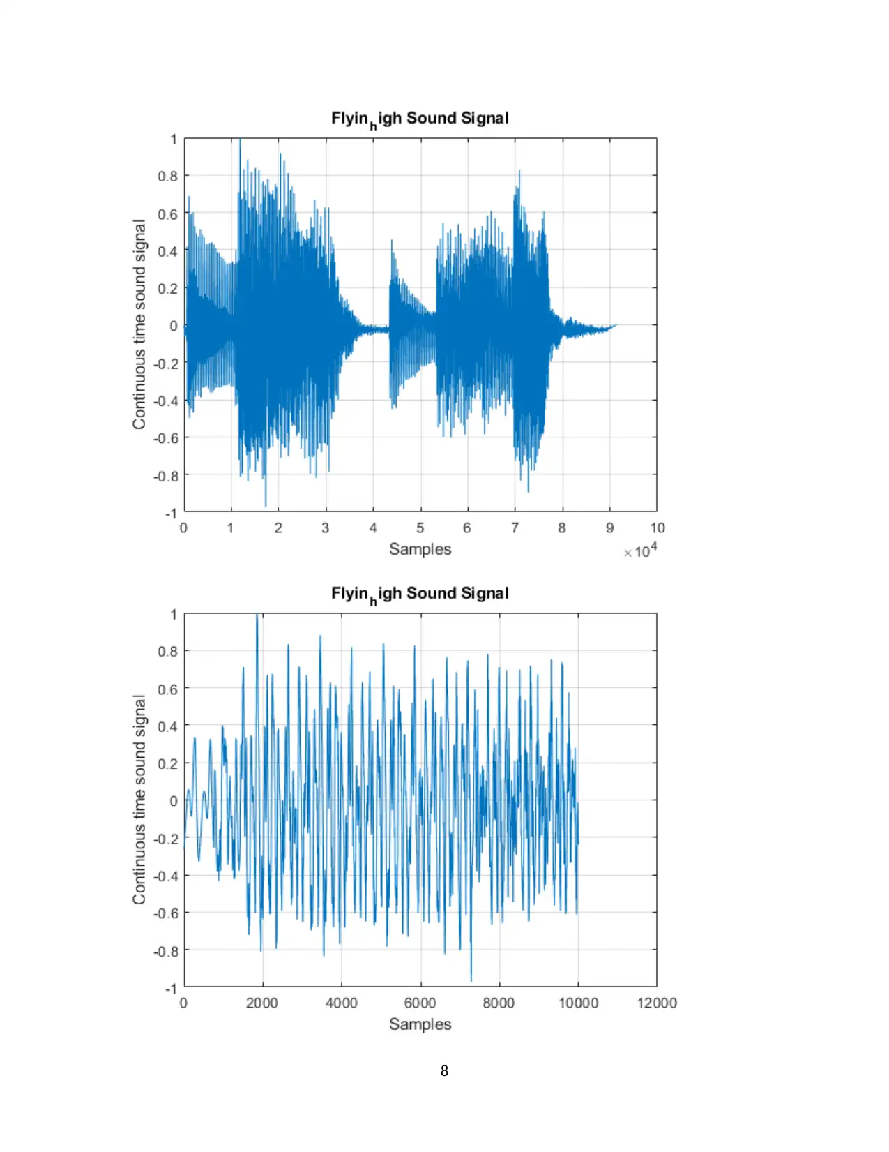
figure(2)
plot(y)
grid on
title('Flyin_high Sound Signal')
xlabel('Samples')
ylabel('Continuous time sound signal')
x=y(10000:20000);
figure(3)
plot(x)
grid on
title('Flyin_high Sound Signal')
xlabel('Samples')
ylabel('Continuous time sound signal')
%Sampling the speech spectrogram
figure(4)
subplot(2,1,1)
specgram(y)
subplot(2,1,2)
specgram(x,256,fs) %outputs the line spectra
7
8
⊘ This is a preview!⊘
Do you want full access?
Subscribe today to unlock all pages.
Trusted by 1+ million students worldwide
PART II (VIDEO PROCESSING)
Question 1
Merits of the BD method over other codecs in the video processing paper cited.
The method has gained fame among other codecs used in the coding efficiency such that
the video codecs have improved on the codec. The reference mode focuses on the range of
quality alongside the bit rates. The BD metrics are used to calculate the bit rates obtained from a
given video obtained at input of a real time live streaming of activities based on the motion
sensor system. The output signal shows that the quality is based on an interpolating curve which
is based on the tested data points.
It is possible to measure the DB rate such that the small spaces between the overlaps are
determined as distortion areas. The performance of the BD metric is better than the MOS and
PSNR as illustrated by the figure 5 in the document. There are several tests carried out so that the
9
Paraphrase This Document
Need a fresh take? Get an instant paraphrase of this document with our AI Paraphraser
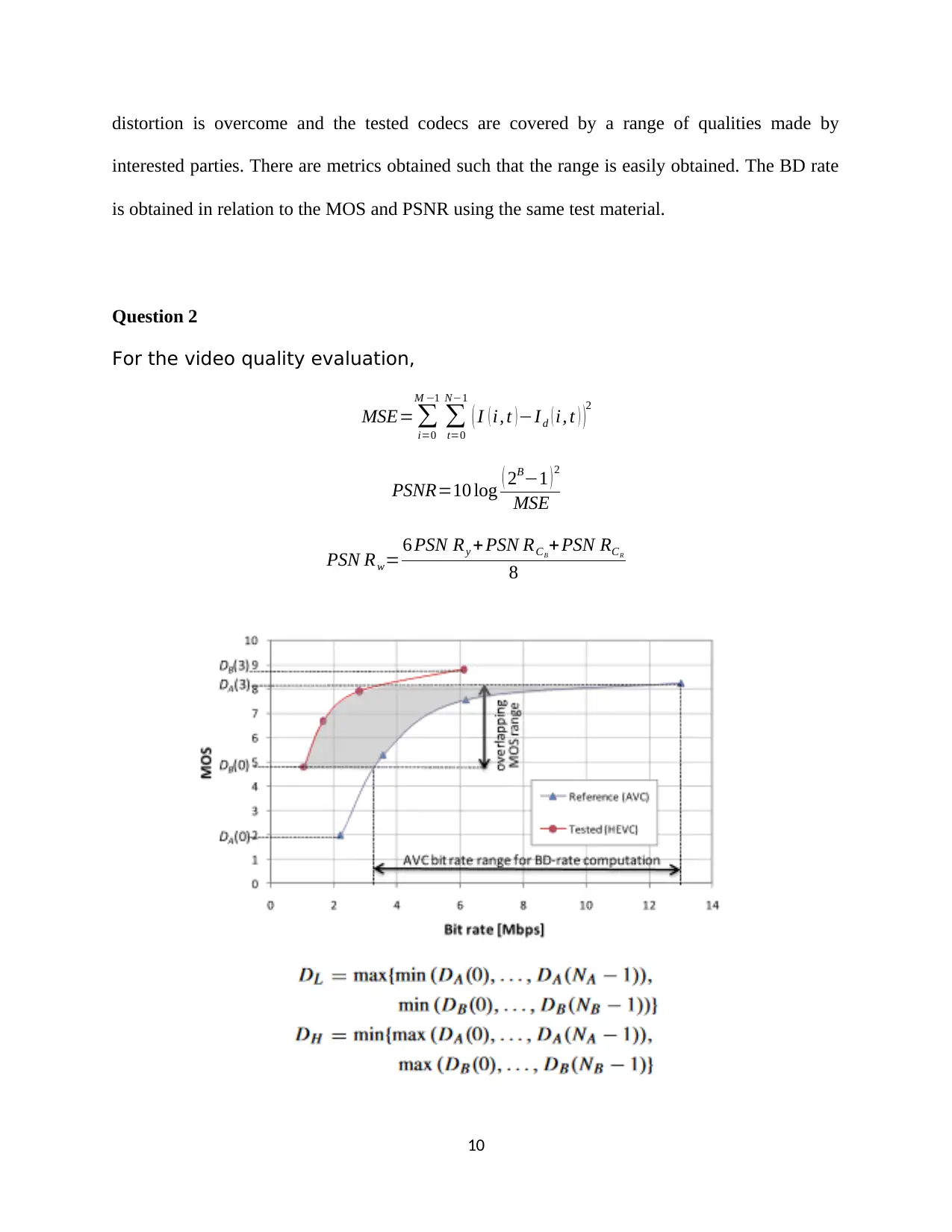
distortion is overcome and the tested codecs are covered by a range of qualities made by
interested parties. There are metrics obtained such that the range is easily obtained. The BD rate
is obtained in relation to the MOS and PSNR using the same test material.
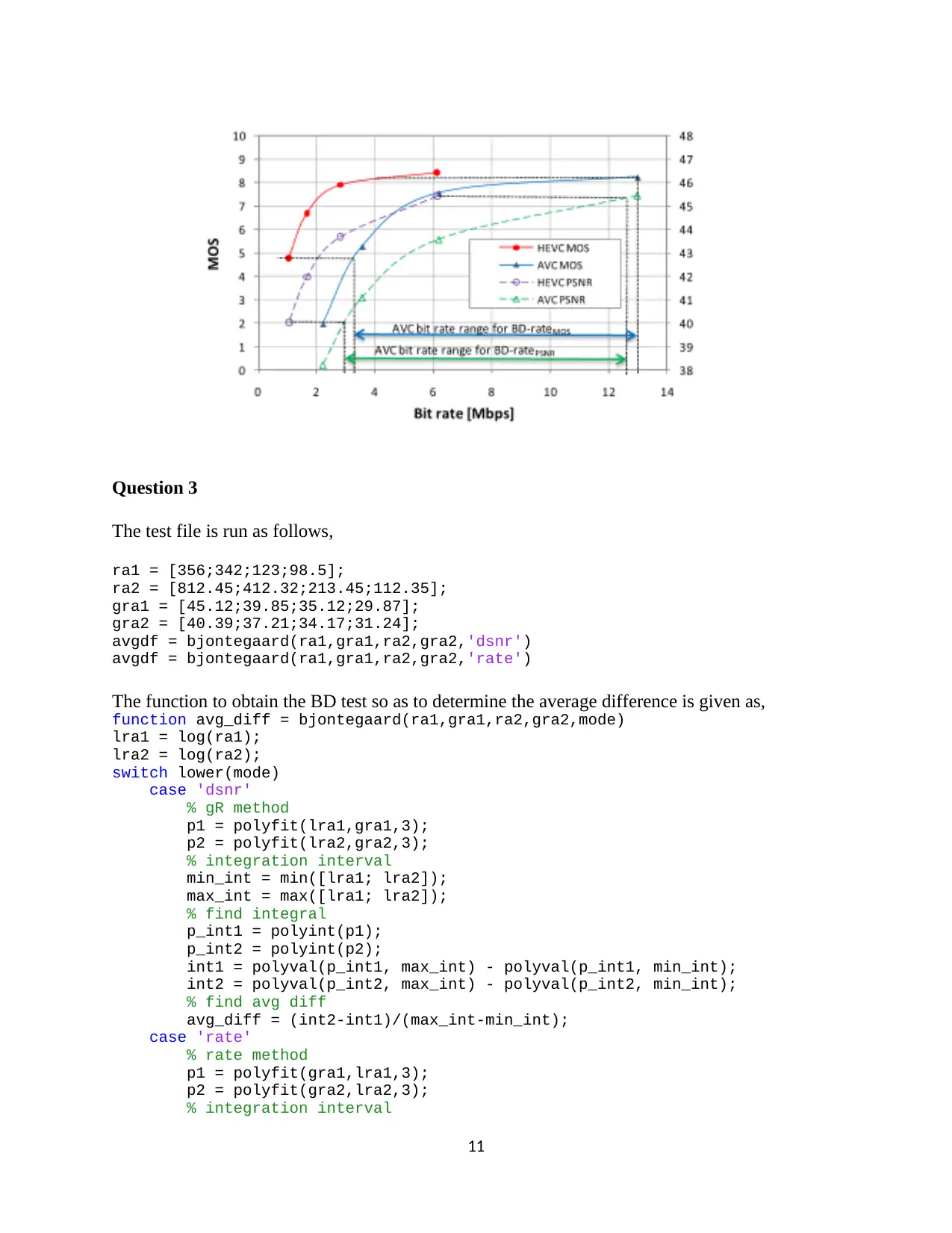
Question 2
For the video quality evaluation,
MSE= ∑
i=0
M −1
∑
t=0
N−1
( I ( i, t )−I d ( i, t ) )2
PSNR=10 log ( 2B−1 ) 2
MSE
PSN Rw= 6 PSN Ry + PSN RCB
+ PSN RCR
8
10
interested parties. There are metrics obtained such that the range is easily obtained. The BD rate
is obtained in relation to the MOS and PSNR using the same test material.
Question 2
For the video quality evaluation,
MSE= ∑
i=0
M −1
∑
t=0
N−1
( I ( i, t )−I d ( i, t ) )2
PSNR=10 log ( 2B−1 ) 2
MSE
PSN Rw= 6 PSN Ry + PSN RCB
+ PSN RCR
8
10
Question 3
The test file is run as follows,
ra1 = [356;342;123;98.5];
ra2 = [812.45;412.32;213.45;112.35];
gra1 = [45.12;39.85;35.12;29.87];
gra2 = [40.39;37.21;34.17;31.24];
avgdf = bjontegaard(ra1,gra1,ra2,gra2,'dsnr')
avgdf = bjontegaard(ra1,gra1,ra2,gra2,'rate')
The function to obtain the BD test so as to determine the average difference is given as,
function avg_diff = bjontegaard(ra1,gra1,ra2,gra2,mode)
lra1 = log(ra1);
lra2 = log(ra2);
switch lower(mode)
case 'dsnr'
% gR method
p1 = polyfit(lra1,gra1,3);
p2 = polyfit(lra2,gra2,3);
% integration interval
min_int = min([lra1; lra2]);
max_int = max([lra1; lra2]);
% find integral
p_int1 = polyint(p1);
p_int2 = polyint(p2);
int1 = polyval(p_int1, max_int) - polyval(p_int1, min_int);
int2 = polyval(p_int2, max_int) - polyval(p_int2, min_int);
% find avg diff
avg_diff = (int2-int1)/(max_int-min_int);
case 'rate'
% rate method
p1 = polyfit(gra1,lra1,3);
p2 = polyfit(gra2,lra2,3);
% integration interval
11
⊘ This is a preview!⊘
Do you want full access?
Subscribe today to unlock all pages.
Trusted by 1+ million students worldwide
1 out of 16
Related Documents


Your All-in-One AI-Powered Toolkit for Academic Success.
+13062052269
info@desklib.com
Available 24*7 on WhatsApp / Email
![[object Object]](/_next/static/media/star-bottom.7253800d.svg)
Unlock your academic potential
Copyright © 2020–2026 A2Z Services. All Rights Reserved. Developed and managed by ZUCOL.