Dynamic Analysis Report: Blast Loading on I-Beam using FEA Methods

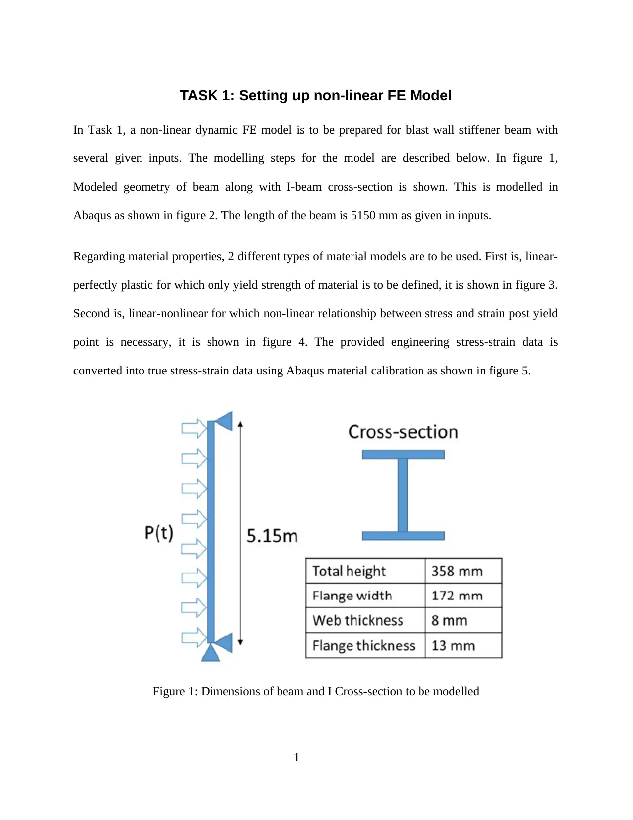
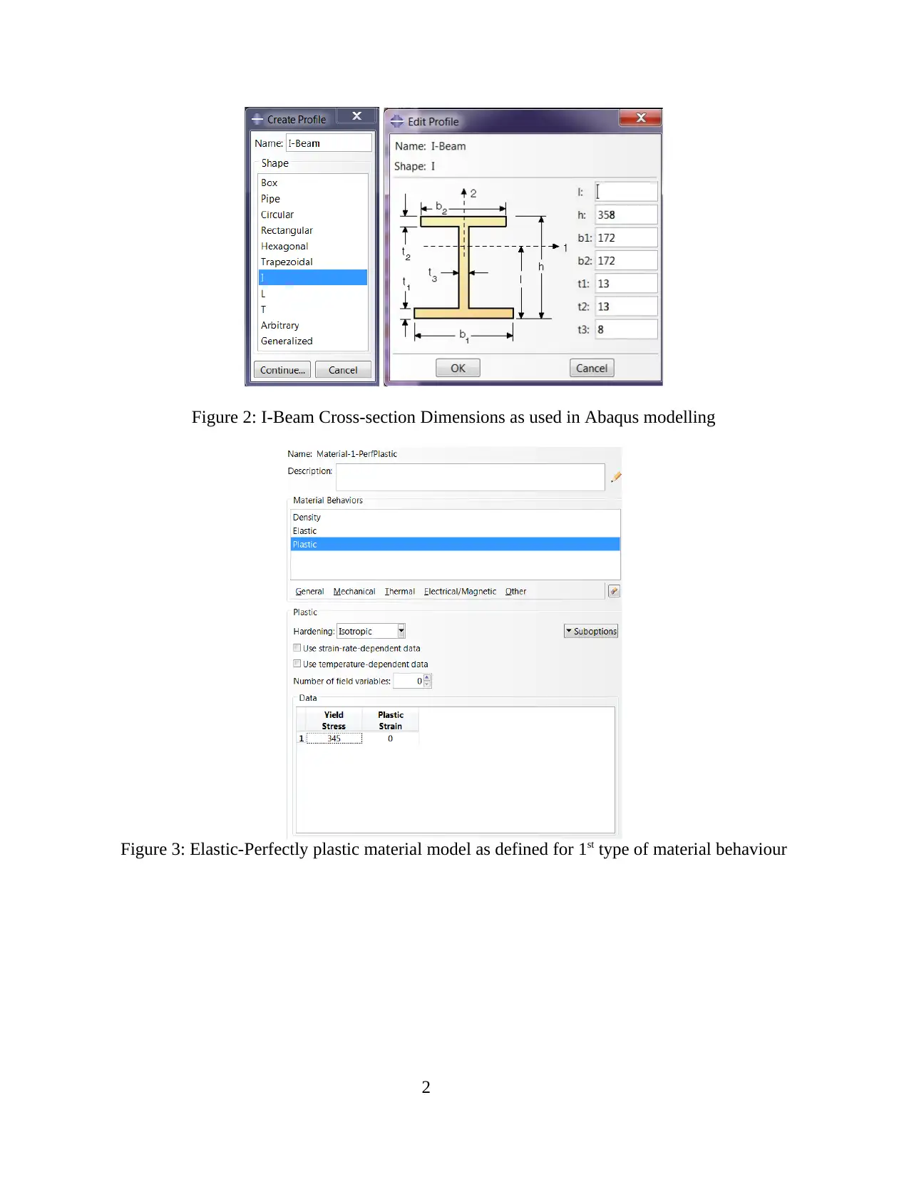
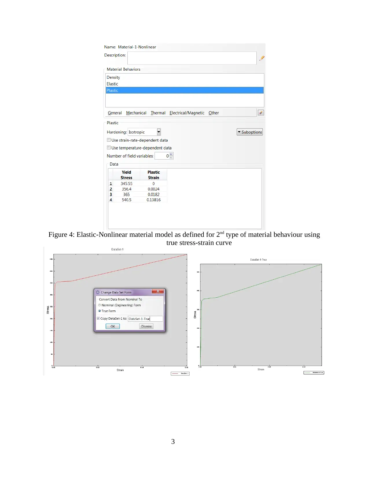
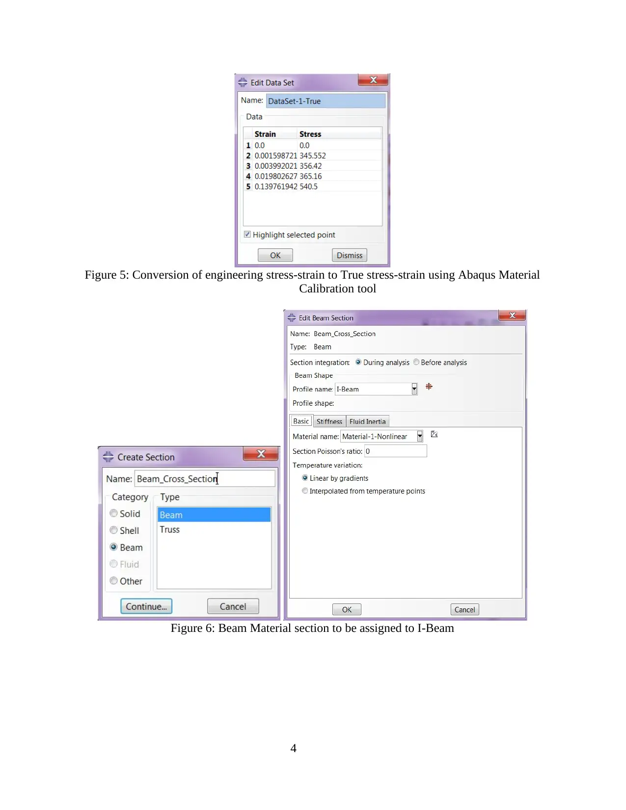
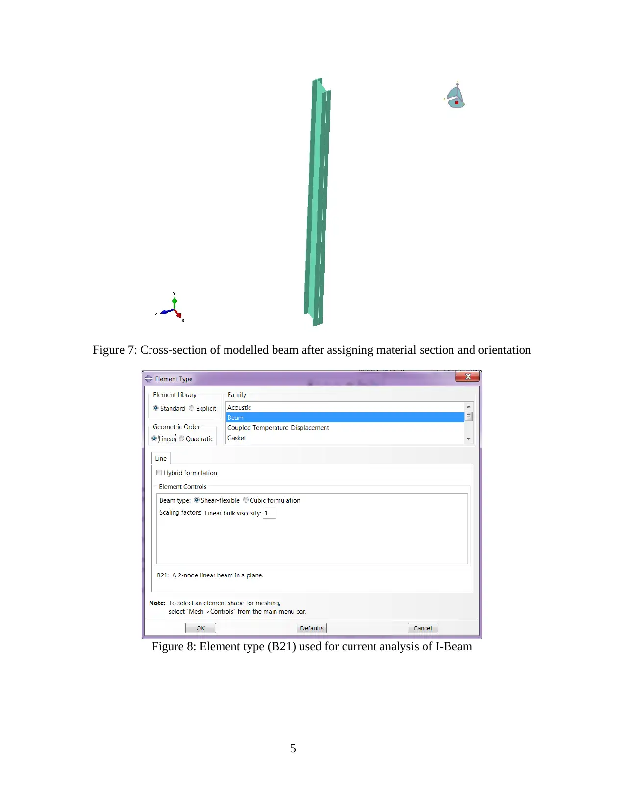
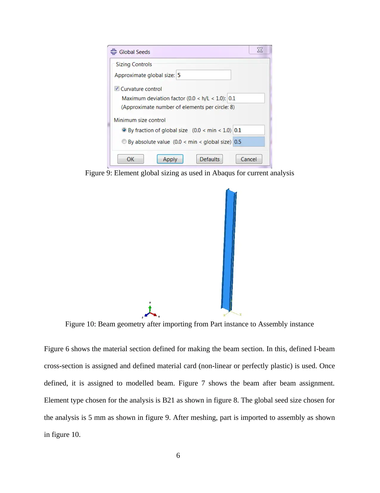
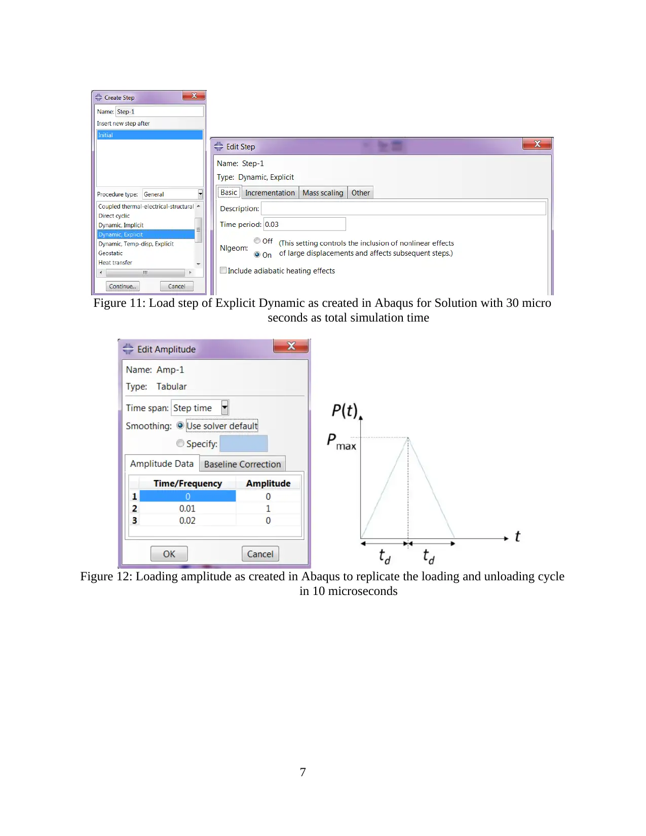
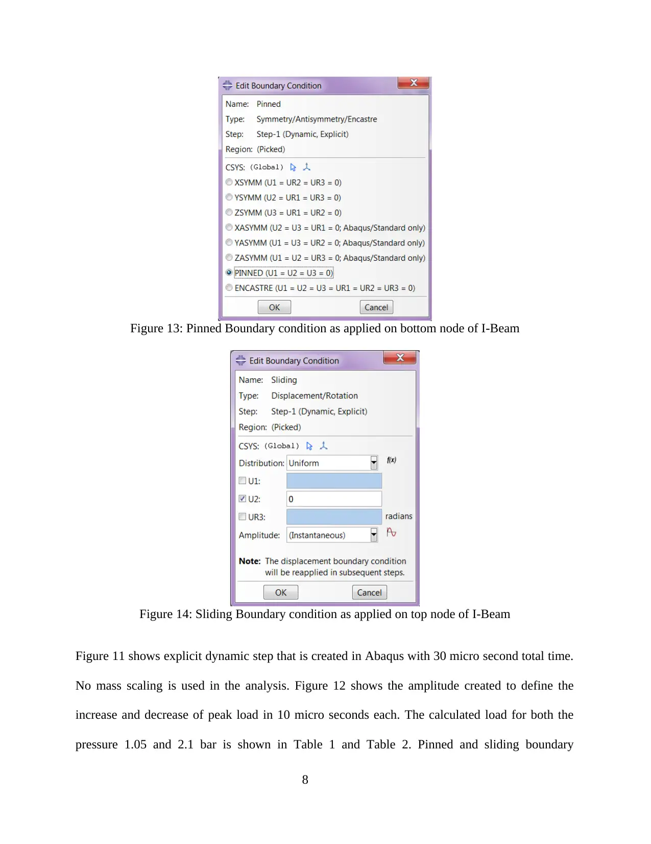
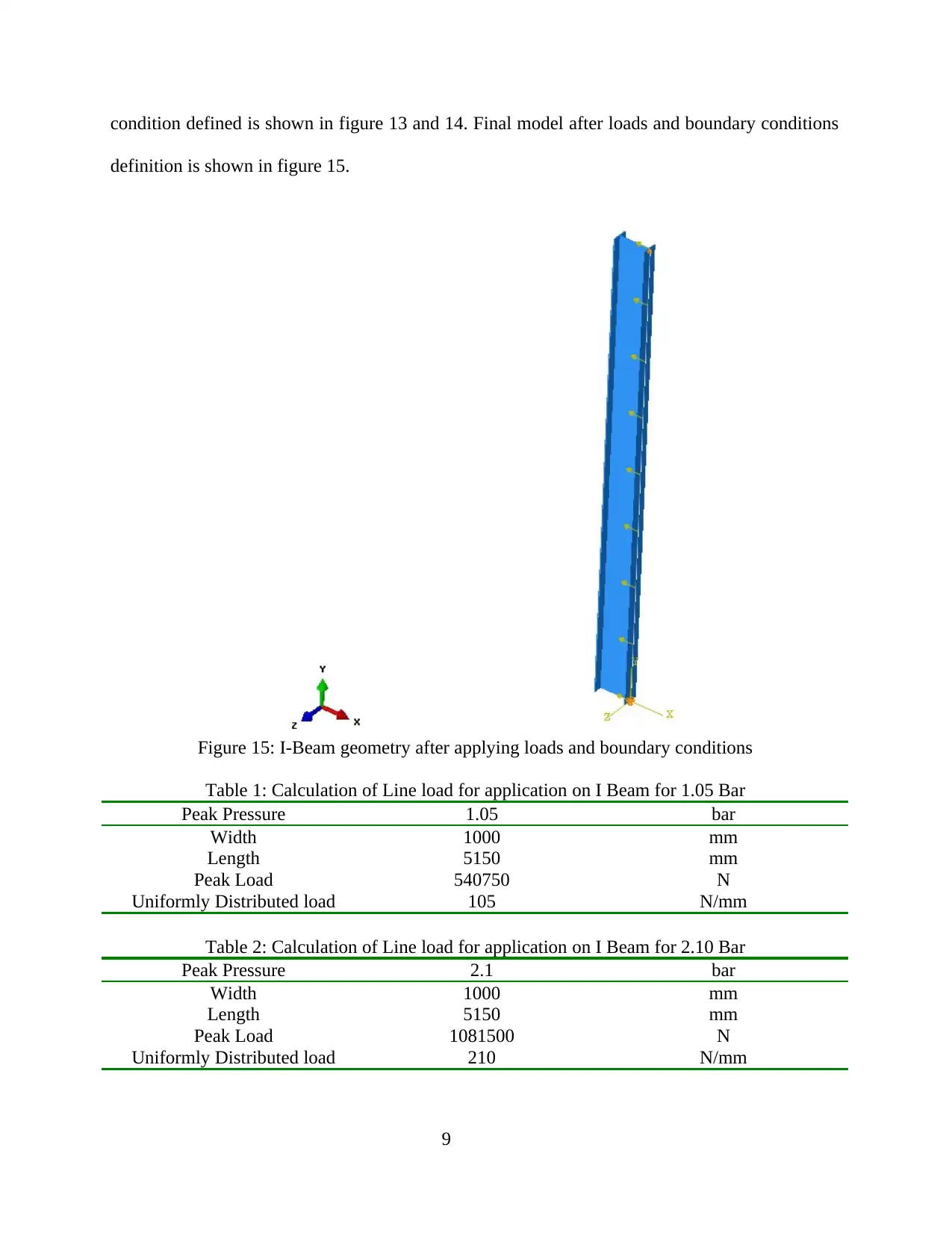
This report details a finite element analysis (FEA) of an I-beam subjected to blast loading, conducted using Abaqus. The study involves creating a non-linear dynamic FE model, defining material properties (linear-perfectly plastic and linear-nonlinear), and applying blast loads. The analysis explores diff...Read More

Dynamic Analysis using blast loading on an I-
Beam using Finite Element methods in Abaqus
<Student Name>
<Student Number>
Assignment Report
Supervisor: <XXX>
Department Name
University Name
<Month Year>

TABLE OF CONTENTS
TABLE OF CONTENTS..................................................................................................................i
TASK 1: Setting up non-linear FE Model.......................................................................................1
TASK 2: Results Of non-linear analysis and Comparison with Biggs-data..................................11
TASK 3: Results Of non-linear analysis with both ends pinned...................................................15
TASK 4: Using Strain rate dependence in Non-linear material.....................................................18
i

TASK 1: Setting up non-linear FE Model
In Task 1, a non-linear dynamic FE model is to be prepared for blast wall stiffener beam with
several given inputs. The modelling steps for the model are described below. In figure 1,
Modeled geometry of beam along with I-beam cross-section is shown. This is modelled in
Abaqus as shown in figure 2. The length of the beam is 5150 mm as given in inputs.
Regarding material properties, 2 different types of material models are to be used. First is, linear-
perfectly plastic for which only yield strength of material is to be defined, it is shown in figure 3.
Second is, linear-nonlinear for which non-linear relationship between stress and strain post yield
point is necessary, it is shown in figure 4. The provided engineering stress-strain data is
converted into true stress-strain data using Abaqus material calibration as shown in figure 5.
Figure 1: Dimensions of beam and I Cross-section to be modelled
1

Figure 2: I-Beam Cross-section Dimensions as used in Abaqus modelling
Figure 3: Elastic-Perfectly plastic material model as defined for 1st type of material behaviour
2

Figure 4: Elastic-Nonlinear material model as defined for 2nd type of material behaviour using
true stress-strain curve
3

Figure 5: Conversion of engineering stress-strain to True stress-strain using Abaqus Material
Calibration tool
Figure 6: Beam Material section to be assigned to I-Beam
4

Figure 7: Cross-section of modelled beam after assigning material section and orientation
Figure 8: Element type (B21) used for current analysis of I-Beam
5

Figure 9: Element global sizing as used in Abaqus for current analysis
Figure 10: Beam geometry after importing from Part instance to Assembly instance
Figure 6 shows the material section defined for making the beam section. In this, defined I-beam
cross-section is assigned and defined material card (non-linear or perfectly plastic) is used. Once
defined, it is assigned to modelled beam. Figure 7 shows the beam after beam assignment.
Element type chosen for the analysis is B21 as shown in figure 8. The global seed size chosen for
the analysis is 5 mm as shown in figure 9. After meshing, part is imported to assembly as shown
in figure 10.
6

Figure 11: Load step of Explicit Dynamic as created in Abaqus for Solution with 30 micro
seconds as total simulation time
Figure 12: Loading amplitude as created in Abaqus to replicate the loading and unloading cycle
in 10 microseconds
7

Figure 13: Pinned Boundary condition as applied on bottom node of I-Beam
Figure 14: Sliding Boundary condition as applied on top node of I-Beam
Figure 11 shows explicit dynamic step that is created in Abaqus with 30 micro second total time.
No mass scaling is used in the analysis. Figure 12 shows the amplitude created to define the
increase and decrease of peak load in 10 micro seconds each. The calculated load for both the
pressure 1.05 and 2.1 bar is shown in Table 1 and Table 2. Pinned and sliding boundary
8

condition defined is shown in figure 13 and 14. Final model after loads and boundary conditions
definition is shown in figure 15.
Figure 15: I-Beam geometry after applying loads and boundary conditions
Table 1: Calculation of Line load for application on I Beam for 1.05 Bar
Peak Pressure 1.05 bar
Width 1000 mm
Length 5150 mm
Peak Load 540750 N
Uniformly Distributed load 105 N/mm
Table 2: Calculation of Line load for application on I Beam for 2.10 Bar
Peak Pressure 2.1 bar
Width 1000 mm
Length 5150 mm
Peak Load 1081500 N
Uniformly Distributed load 210 N/mm
9

Justification for choosing current modelling method –
The Beam modelling method in Abaqus is quite accurate and many benchmark studies have been
performed as available in literature where it has been proven that for simpler problems, 1D beam
modelling approach is found to be nearly accurate with certain assumptions.
The choice of linear element is justified by the fact that the mesh convergence study is
performed. Choosing non-linear elements does not change the results hence linear elements are
chosen. Mesh density is justified again with mesh convergence study.
10

TASK 2: Results Of non-linear analysis and Comparison with Biggs-
data
In the current section, Results are discussed. There are 9 different models created which are
shown in figure 16.
Figure 16: Snap of different analysis prepared and solved in Abaqus (Details of analysis names
given in table 3)
Figure 17 compares the displacement for 1.05 bar pressure for 2 different types of material
definition and results are similar. Figure 18 compares the stress which differs significantly,
stresses with non-linear material properties are more realistic and close to reality. Figure 19
compares displacement with 2.1 bar which is comparable while stresses are completely
inaccurate with perfectly plastic and accurate with non-linear material as shown in figure 20.
11

(a) (b)
Figure 17: Comparison of Displacement plots from one end pinned analysis with 1.05 bar peak
pressure using (a) Perfectly plastic material, (b) Non-linear material properties
(a) (b)
Figure 18: Comparison of Stress plots from one end pinned analysis with 1.05 bar peak pressure
using (a) Perfectly plastic material, (b) Non-linear material properties
12

(a) (b)
Figure 19: Comparison of Displacement plots from one end pinned analysis with 2.10 bar peak
pressure using (a) Perfectly plastic material, (b) Non-linear material properties
(a) (b)
Figure 20: Comparison of Stress plots from one end pinned analysis with 2.10 bar peak pressure
using (a) Perfectly plastic material, (b) Non-linear material properties
Figure 21 compares the reaction forces with biggs data and it compares the reaction force
prediction. For initial 25 micro seconds, the reaction plots compares well and after that biggs
prediction are significantly off compared to simulation results.
13

(a)
(b)
Figure 21: Comparison of reaction plot with biggs prediction data (a)From biggs prediction
model, (b) from simulation model
14

TASK 3: Results Of non-linear analysis with both ends pinned
Results with both ends pinned boundary condition are discussed in this section.
Figure 21 compares the displacement for 1.05 bar pressure for 2 different types of material
definition and results are significantly different because perfectly plastic material underestimates
the material strength. Figure 22 compares the stress which differs significantly, stresses with non-
linear material properties are more realistic and close to reality.
Figure 23 compares displacement with 2.1 bar which is higher and more realistic with non-linear
material properties while stresses are also more accurate with non-linear material as shown in
figure 24.
(a) (b)
Figure 22: Comparison of Displacement plots from both end pinned analysis with 1.05 bar peak
pressure using (a) Perfectly plastic material, (b) Non-linear material properties
15

(a) (b)
Figure 23: Comparison of Stress plots from both end pinned analysis with 1.05 bar peak pressure
using (a) Perfectly plastic material, (b) Non-linear material properties
(a) (b)
Figure 24: Comparison of Displacement plots from both end pinned analysis with 2.10 bar peak
pressure using (a) Perfectly plastic material, (b) Non-linear material properties
16

(a) (b)
Figure 25: Comparison of Stress plots from both end pinned analysis with 2.10 bar peak pressure
using (a) Perfectly plastic material, (b) Non-linear material properties
Comparing the results of different boundary conditions, following table is obtained:
Table 3: Comparison of Stress and displacement for different boundary condition
Peak Pressure Boundary condition Stress (MPa) Displacement (mm)
1.05 bar One End Pinned 399.3 534.7
Both ends pinned 76.5 106.1
2.10 bar One End Pinned 534.7 945.9
Both ends pinned 86.5 93.8
Based on the comparison, it can be concluded that both ends pinned results in considerable
reduction in stress and deformation.
17

TASK 4: Using Strain rate dependence in Non-linear material
Defined non-linear material properties are defined with Power law for strain rate dependence as
shown in figure 25. Figure 26 and 27 shows the stress and displacement obtained from the
analysis. As compared to material definition without strain rate dependence, no different in
results was observed with strain rate dependence included in material properties.
Figure 26: Strain rate dependence using power law as defined in Non-linear material properties
of Abaqus with given values
18

Figure 27: Stress plots from both end pinned analysis with 2.10 bar peak pressure using Non-
linear Strain rate dependent material properties
Figure 28: Displacement plots from both end pinned analysis with 2.10 bar peak pressure using
Non-linear Strain rate dependent material properties
19

Table 4: Comparison of Stress and displacement for with and without strain rate effect
Peak Pressure Material condition Stress (MPa) Displacement (mm)
2.10 bar
Without strain rate
effect in material
534.7 945.9
With strain rate
effect in material
534.8 945.9
As can be seen from Table 4, there is no evidence of strain rate effect on the results of beam as
obtained from simulation.
20