University Assignment: Dynamic Lot Sizing Case Study and Analysis

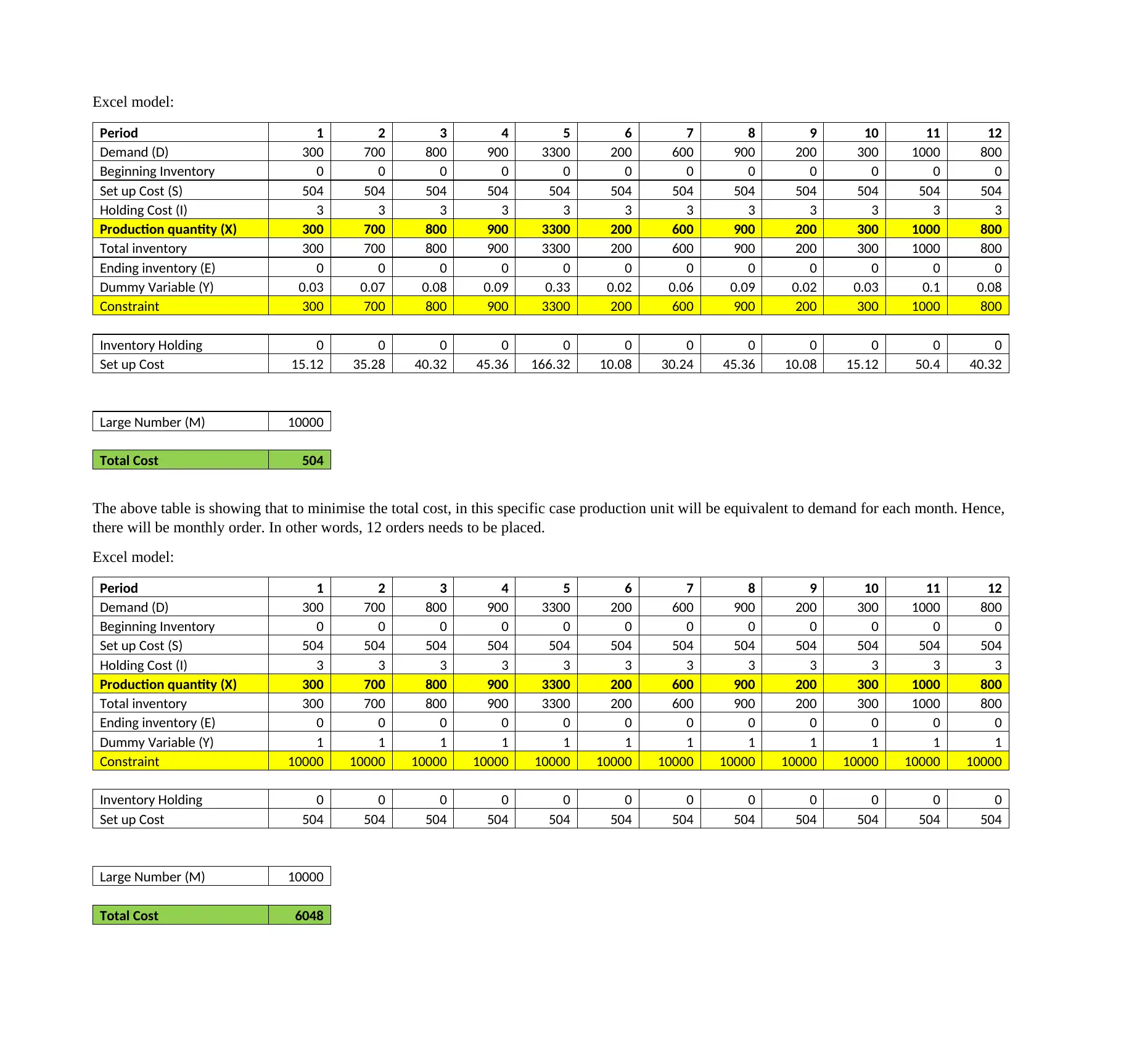
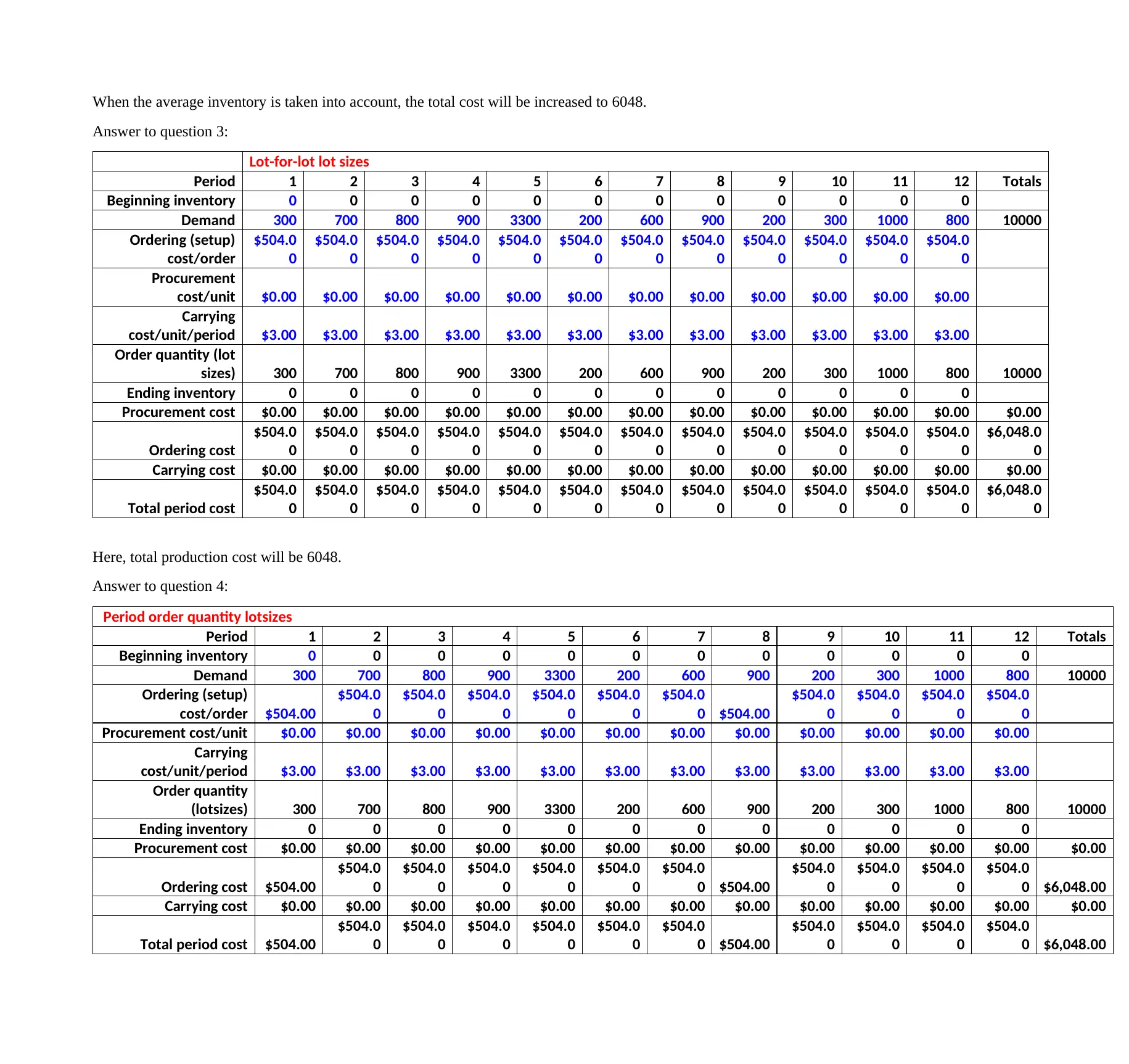
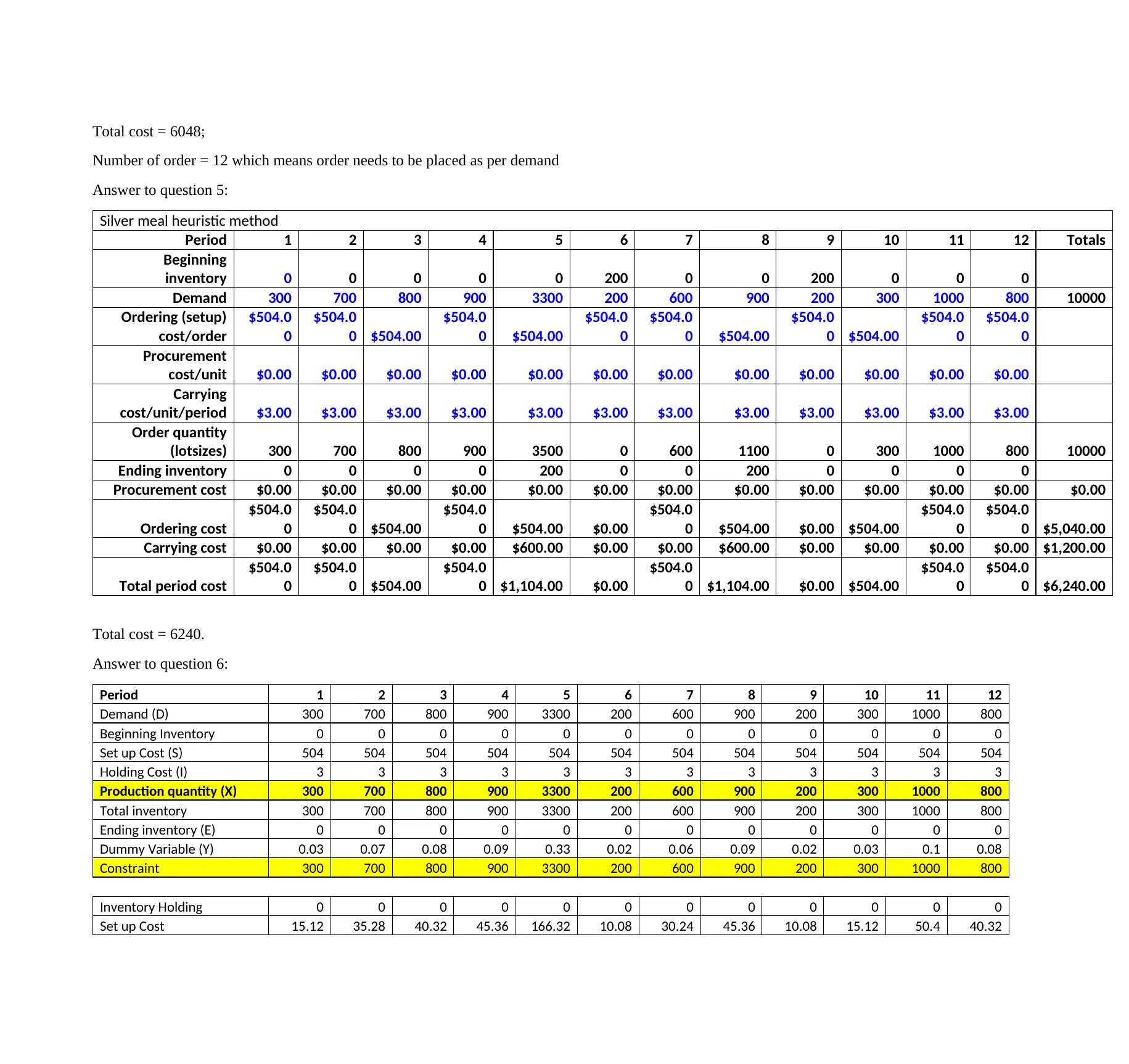
This case study analyzes dynamic lot sizing, a crucial aspect of inventory management when demand varies over time. The solution begins with an Economic Order Quantity (EOQ) calculation to determine the optimal order quantity, followed by the total cost, frequency of orders, and time between orders. The case study then explores different lot-sizing methods, including a period-by-period analysis using an Excel model to minimize total costs. It examines lot-for-lot and Silver Meal heuristic methods, providing detailed calculations for each period, including ordering costs, carrying costs, and total production costs. The analysis considers constraints such as ordering costs, production quantities, ending inventory, and dummy variables, offering a comprehensive understanding of dynamic lot sizing techniques.

Assignment 1 - Case Study (Individual Assignment)
Name of the Student
Name Of the University
Author Note

Answer to question 1:
Annual demand = 10000
Ordering cost = $504
Holding cost = $3
Optimal order quantity (EOQ) = sqrt(2*504*10000/3) = 1833
Now, total cost = annual ordering cost + annual holding cost
= (10000/1833)*504 + (1833/2)*3
=$5499.09
Frequency of orders = 10000/1833 = 5.46 = 6 times
Time between orders = 12/6 = 2 months
Answer to question 2:
Let St is the set up cost or ordering cost in period t
It is the inventory holding cost in period t
Dt is the demand in period t
Xt is the production quantity in period t
Yt is dummy variable representing 1, if Xt >0, else 0
M is very large number
Et is ending inventory in period t carried to next period
Therefore, the objective function will be:
Min = ∑
t =1
12
( I¿ ¿ t∗Et +Y t∗St )¿
Constraints:
Ordering Cost = M Y t ≥ Xt
Production quantity = Xt ≥ 0
Ending Inventory = Et ≥ 0
Production quantity = Xt =Integer
Dummy variable = Y t =binary

Excel model:
Period 1 2 3 4 5 6 7 8 9 10 11 12
Demand (D) 300 700 800 900 3300 200 600 900 200 300 1000 800
Beginning Inventory 0 0 0 0 0 0 0 0 0 0 0 0
Set up Cost (S) 504 504 504 504 504 504 504 504 504 504 504 504
Holding Cost (I) 3 3 3 3 3 3 3 3 3 3 3 3
Production quantity (X) 300 700 800 900 3300 200 600 900 200 300 1000 800
Total inventory 300 700 800 900 3300 200 600 900 200 300 1000 800
Ending inventory (E) 0 0 0 0 0 0 0 0 0 0 0 0
Dummy Variable (Y) 0.03 0.07 0.08 0.09 0.33 0.02 0.06 0.09 0.02 0.03 0.1 0.08
Constraint 300 700 800 900 3300 200 600 900 200 300 1000 800
Inventory Holding 0 0 0 0 0 0 0 0 0 0 0 0
Set up Cost 15.12 35.28 40.32 45.36 166.32 10.08 30.24 45.36 10.08 15.12 50.4 40.32
Large Number (M) 10000
Total Cost 504
The above table is showing that to minimise the total cost, in this specific case production unit will be equivalent to demand for each month. Hence,
there will be monthly order. In other words, 12 orders needs to be placed.
Excel model:
Period 1 2 3 4 5 6 7 8 9 10 11 12
Demand (D) 300 700 800 900 3300 200 600 900 200 300 1000 800
Beginning Inventory 0 0 0 0 0 0 0 0 0 0 0 0
Set up Cost (S) 504 504 504 504 504 504 504 504 504 504 504 504
Holding Cost (I) 3 3 3 3 3 3 3 3 3 3 3 3
Production quantity (X) 300 700 800 900 3300 200 600 900 200 300 1000 800
Total inventory 300 700 800 900 3300 200 600 900 200 300 1000 800
Ending inventory (E) 0 0 0 0 0 0 0 0 0 0 0 0
Dummy Variable (Y) 1 1 1 1 1 1 1 1 1 1 1 1
Constraint 10000 10000 10000 10000 10000 10000 10000 10000 10000 10000 10000 10000
Inventory Holding 0 0 0 0 0 0 0 0 0 0 0 0
Set up Cost 504 504 504 504 504 504 504 504 504 504 504 504
Large Number (M) 10000
Total Cost 6048

When the average inventory is taken into account, the total cost will be increased to 6048.
Answer to question 3:
Lot-for-lot lot sizes
Period 1 2 3 4 5 6 7 8 9 10 11 12 Totals
Beginning inventory 0 0 0 0 0 0 0 0 0 0 0 0
Demand 300 700 800 900 3300 200 600 900 200 300 1000 800 10000
Ordering (setup)
cost/order
$504.0
0
$504.0
0
$504.0
0
$504.0
0
$504.0
0
$504.0
0
$504.0
0
$504.0
0
$504.0
0
$504.0
0
$504.0
0
$504.0
0
Procurement
cost/unit $0.00 $0.00 $0.00 $0.00 $0.00 $0.00 $0.00 $0.00 $0.00 $0.00 $0.00 $0.00
Carrying
cost/unit/period $3.00 $3.00 $3.00 $3.00 $3.00 $3.00 $3.00 $3.00 $3.00 $3.00 $3.00 $3.00
Order quantity (lot
sizes) 300 700 800 900 3300 200 600 900 200 300 1000 800 10000
Ending inventory 0 0 0 0 0 0 0 0 0 0 0 0
Procurement cost $0.00 $0.00 $0.00 $0.00 $0.00 $0.00 $0.00 $0.00 $0.00 $0.00 $0.00 $0.00 $0.00
Ordering cost
$504.0
0
$504.0
0
$504.0
0
$504.0
0
$504.0
0
$504.0
0
$504.0
0
$504.0
0
$504.0
0
$504.0
0
$504.0
0
$504.0
0
$6,048.0
0
Carrying cost $0.00 $0.00 $0.00 $0.00 $0.00 $0.00 $0.00 $0.00 $0.00 $0.00 $0.00 $0.00 $0.00
Total period cost
$504.0
0
$504.0
0
$504.0
0
$504.0
0
$504.0
0
$504.0
0
$504.0
0
$504.0
0
$504.0
0
$504.0
0
$504.0
0
$504.0
0
$6,048.0
0
Here, total production cost will be 6048.
Answer to question 4:
Period order quantity lotsizes
Period 1 2 3 4 5 6 7 8 9 10 11 12 Totals
Beginning inventory 0 0 0 0 0 0 0 0 0 0 0 0
Demand 300 700 800 900 3300 200 600 900 200 300 1000 800 10000
Ordering (setup)
cost/order $504.00
$504.0
0
$504.0
0
$504.0
0
$504.0
0
$504.0
0
$504.0
0 $504.00
$504.0
0
$504.0
0
$504.0
0
$504.0
0
Procurement cost/unit $0.00 $0.00 $0.00 $0.00 $0.00 $0.00 $0.00 $0.00 $0.00 $0.00 $0.00 $0.00
Carrying
cost/unit/period $3.00 $3.00 $3.00 $3.00 $3.00 $3.00 $3.00 $3.00 $3.00 $3.00 $3.00 $3.00
Order quantity
(lotsizes) 300 700 800 900 3300 200 600 900 200 300 1000 800 10000
Ending inventory 0 0 0 0 0 0 0 0 0 0 0 0
Procurement cost $0.00 $0.00 $0.00 $0.00 $0.00 $0.00 $0.00 $0.00 $0.00 $0.00 $0.00 $0.00 $0.00
Ordering cost $504.00
$504.0
0
$504.0
0
$504.0
0
$504.0
0
$504.0
0
$504.0
0 $504.00
$504.0
0
$504.0
0
$504.0
0
$504.0
0 $6,048.00
Carrying cost $0.00 $0.00 $0.00 $0.00 $0.00 $0.00 $0.00 $0.00 $0.00 $0.00 $0.00 $0.00 $0.00
Total period cost $504.00
$504.0
0
$504.0
0
$504.0
0
$504.0
0
$504.0
0
$504.0
0 $504.00
$504.0
0
$504.0
0
$504.0
0
$504.0
0 $6,048.00

Total cost = 6048;
Number of order = 12 which means order needs to be placed as per demand
Answer to question 5:
Silver meal heuristic method
Period 1 2 3 4 5 6 7 8 9 10 11 12 Totals
Beginning
inventory 0 0 0 0 0 200 0 0 200 0 0 0
Demand 300 700 800 900 3300 200 600 900 200 300 1000 800 10000
Ordering (setup)
cost/order
$504.0
0
$504.0
0 $504.00
$504.0
0 $504.00
$504.0
0
$504.0
0 $504.00
$504.0
0 $504.00
$504.0
0
$504.0
0
Procurement
cost/unit $0.00 $0.00 $0.00 $0.00 $0.00 $0.00 $0.00 $0.00 $0.00 $0.00 $0.00 $0.00
Carrying
cost/unit/period $3.00 $3.00 $3.00 $3.00 $3.00 $3.00 $3.00 $3.00 $3.00 $3.00 $3.00 $3.00
Order quantity
(lotsizes) 300 700 800 900 3500 0 600 1100 0 300 1000 800 10000
Ending inventory 0 0 0 0 200 0 0 200 0 0 0 0
Procurement cost $0.00 $0.00 $0.00 $0.00 $0.00 $0.00 $0.00 $0.00 $0.00 $0.00 $0.00 $0.00 $0.00
Ordering cost
$504.0
0
$504.0
0 $504.00
$504.0
0 $504.00 $0.00
$504.0
0 $504.00 $0.00 $504.00
$504.0
0
$504.0
0 $5,040.00
Carrying cost $0.00 $0.00 $0.00 $0.00 $600.00 $0.00 $0.00 $600.00 $0.00 $0.00 $0.00 $0.00 $1,200.00
Total period cost
$504.0
0
$504.0
0 $504.00
$504.0
0 $1,104.00 $0.00
$504.0
0 $1,104.00 $0.00 $504.00
$504.0
0
$504.0
0 $6,240.00
Total cost = 6240.
Answer to question 6:
Period 1 2 3 4 5 6 7 8 9 10 11 12
Demand (D) 300 700 800 900 3300 200 600 900 200 300 1000 800
Beginning Inventory 0 0 0 0 0 0 0 0 0 0 0 0
Set up Cost (S) 504 504 504 504 504 504 504 504 504 504 504 504
Holding Cost (I) 3 3 3 3 3 3 3 3 3 3 3 3
Production quantity (X) 300 700 800 900 3300 200 600 900 200 300 1000 800
Total inventory 300 700 800 900 3300 200 600 900 200 300 1000 800
Ending inventory (E) 0 0 0 0 0 0 0 0 0 0 0 0
Dummy Variable (Y) 0.03 0.07 0.08 0.09 0.33 0.02 0.06 0.09 0.02 0.03 0.1 0.08
Constraint 300 700 800 900 3300 200 600 900 200 300 1000 800
Inventory Holding 0 0 0 0 0 0 0 0 0 0 0 0
Set up Cost 15.12 35.28 40.32 45.36 166.32 10.08 30.24 45.36 10.08 15.12 50.4 40.32

Large Number (M) 10000
Total Cost 504
In case of use of traditional method, then also it is found that the total cost will be 504 and the number of order placed will be 12 which is equivalent to
demand for each month.