Analysis of Dynamic Lot Sizing Methods in Inventory Management

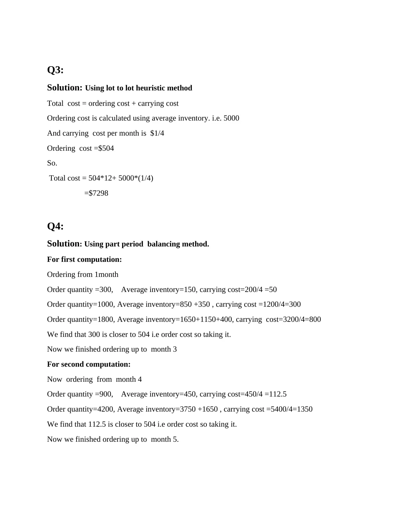
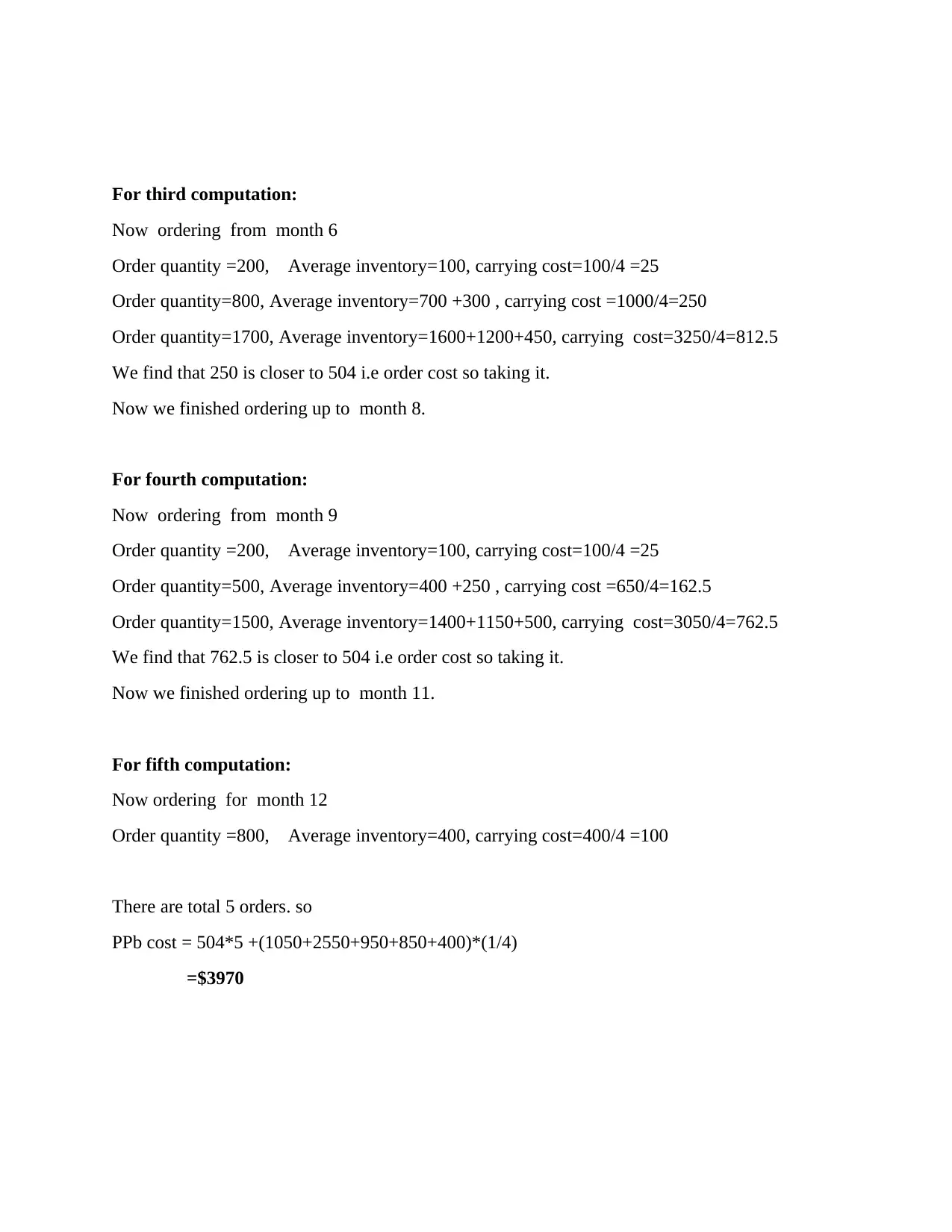
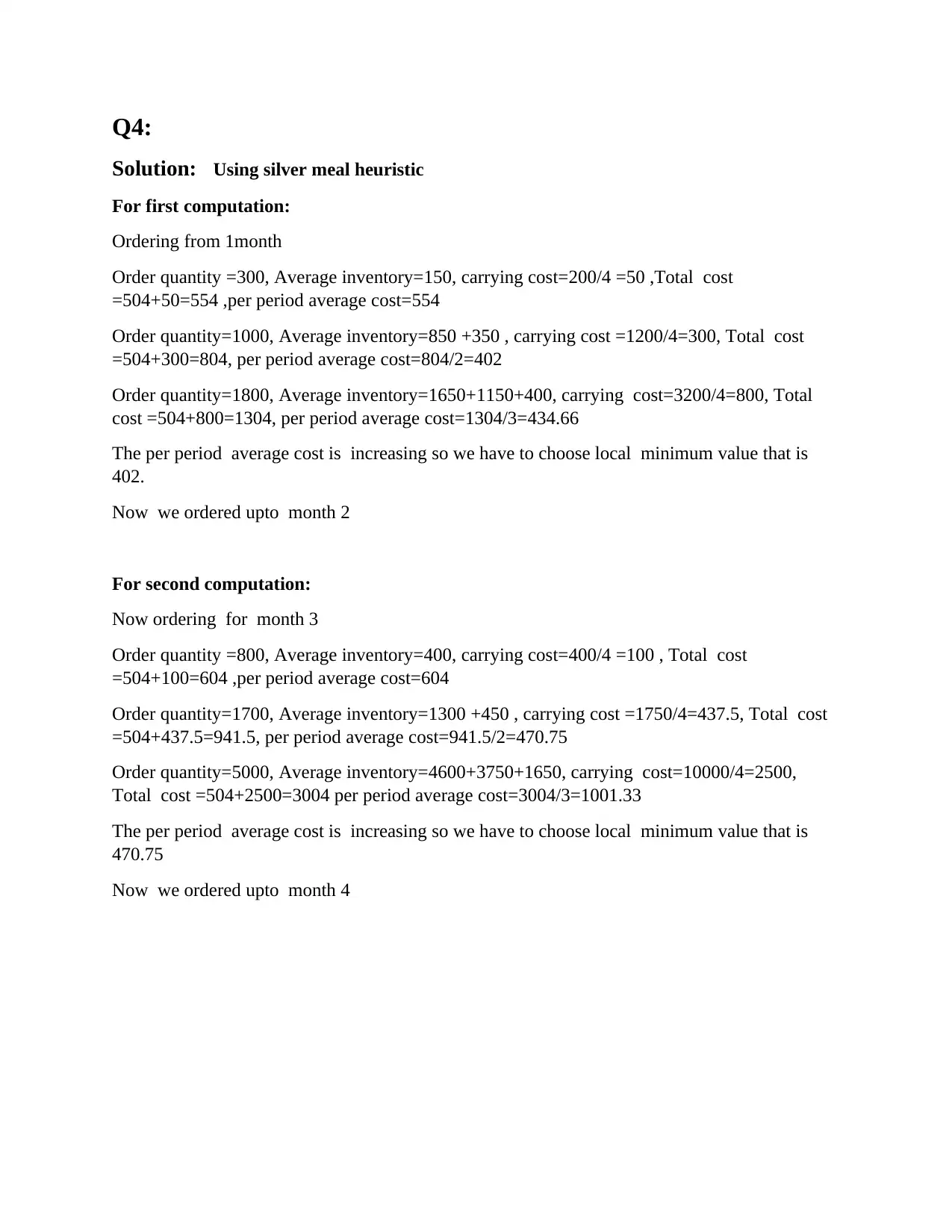
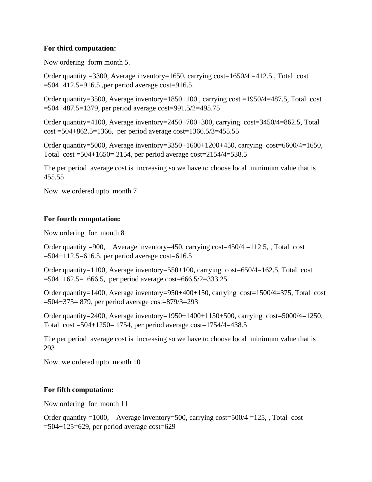
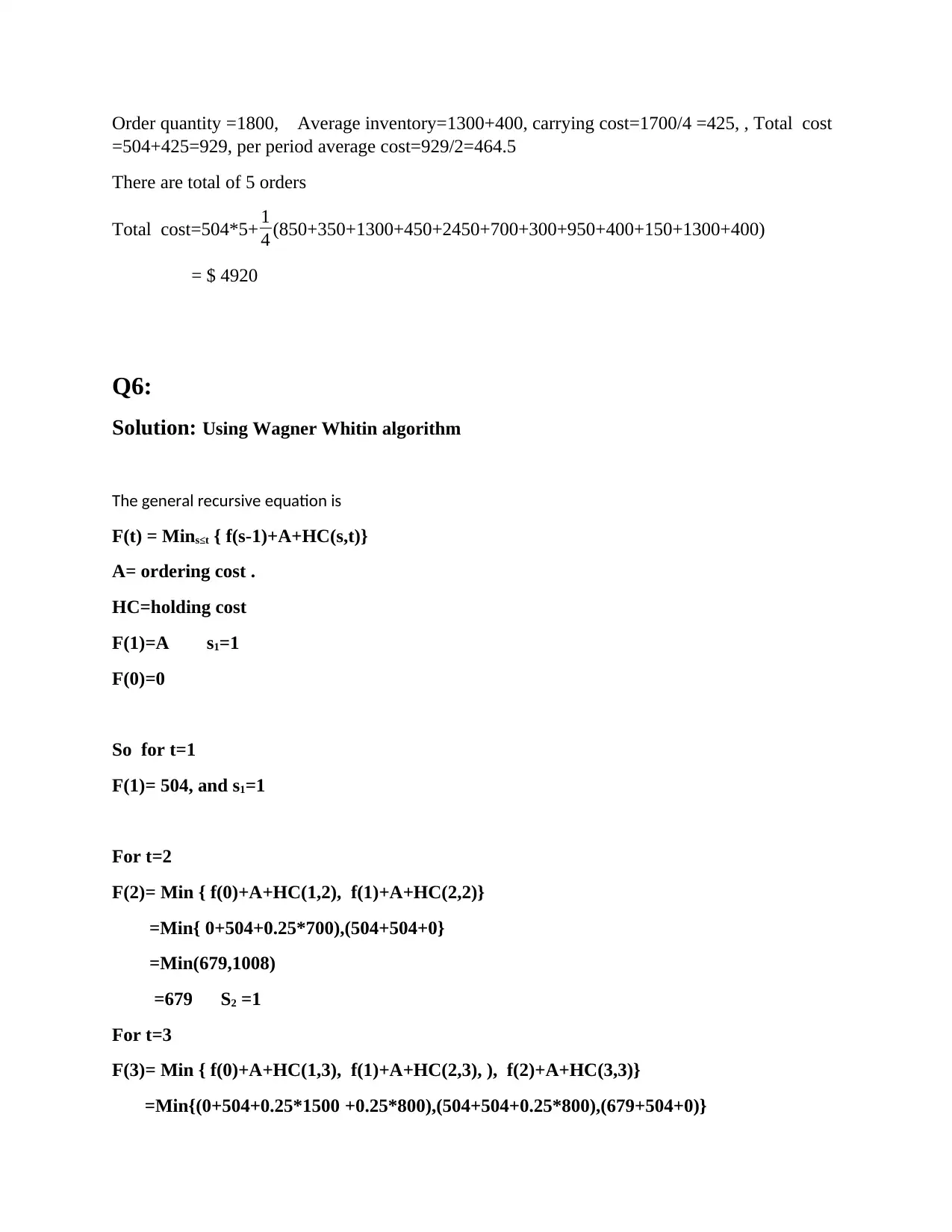
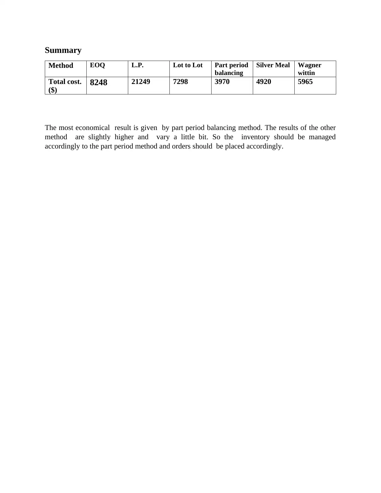
This assignment provides a comprehensive analysis of dynamic lot sizing methods in inventory management. It begins with a solution for optimal order quantity using the Economic Order Quantity (EOQ) model, followed by the development of a mathematical model for dynamic demand across twelve months, solved using Excel Solver. The analysis extends to comparing various heuristic methods like Lot-to-Lot, Part Period Balancing, Silver Meal, and the Wagner-Whitin algorithm to determine the most cost-effective approach for managing inventory with time-varying demand. The study concludes that the Part Period Balancing method yields the most economical results, providing a practical recommendation for inventory management based on the comparative cost analysis of different lot sizing techniques.

Questions
Q1
Solution:
 Optimal order quantity: = √ 2 × D × K
H
K= Annual demand=10,000 units
H=Annual holding cost per unit = $3
D=Fixed cost per year= $504
Optimal order quantity= √ 2 ×504 × 10000
3
= 1833 units.
 Total cost = ordering cost + holding cost
= $ 504* number of orders per year( =5.456) +1833 *3
=$ 8248.82
 Number of orders/ frequency of orders = D
EOQ
= 10000
1833
= 5.456
 Time between orders = EOQ/ D = 1833/10000=0.1833 year
= 0.1833 *13
=2.19 months
Q2.

Solutions:
(a)The demands received in the months are shown in the table:
Months 1 2 3 4 5 6 7 8 9 10 11 12
Demand 300 700 800 900 3300 200 600 900 200 300 1000 800
Development of mathematical model:
Assuming:
Yi =1 ; denotes if an order is placed in ith month. (i.e. 0 for order is not placed and 1for order is
placed).
Xi = denotes the ordered quantity in ith month.
Ordering cost per order is: $504
Holding cost per order per month = $ 3
number of months (12)
=$ 1
4
Ii =denotes the ending inventory at the time of ith month.
The holding cost is applied to ending inventory.
The total cost is calculated as = ∑
i=1
n
504 Y i+ 1
4 ( I1 + I2 + I3 … .. … .+ I12)
I12 is 0 because the at last inventory gets empty.
Now looking at constraints:
 X1 ≥ D1 means ordered quantity should be greater than the demand for first month.
Also I1 = X1 – D1 ; The orders left are equal to the ending inventory.
 X1 +X2 ≥ D1 + D2 means ordered quantity in first two months should be greater than
cumulative demand in the first two months. Also I2 = X1 + X2 – D1 – D2
Similarly there are 12 constraint equations
From these we can write : ∑
i=1
n
Xi ≥ ∑
i=1
n
Y i
Now there are 12 more constraints arises for relating Xi , Yi ; as
Xi ≤ M Yi (where M is a constant) this will for the order quantity to be zero in month when
there in no order placed;

Now on putting the values of ending inventories which we get from constraint on the total cost
function ;(i.e. I1 , I2 etc)
The total cost is calculated as =
∑
i=1
n
504 Y i+ 1
4 ( ( 12 X1 +11 X2+10 X3 … .. … .+X12 )− ( 12 D1 +11 D2+10 D3 … ..… .+D12 ) )
The demand term is the constant term which we can remove for linear programming:
So minimize :
∑
i=1
n
504 Y i+ 1
4 ( ( 12 X1 +11 X2+10 X3 … .. … .+ X12 ) )
The excel solver gives the result
Months Demand coefficentsConstraints Xi ≤ M Yi
1 300 1 1000 12 10000
2 700 0 0 11 0
3 800 1 1700 10 10000
4 900 0 0 9 0
5 3300 1 3300 8 10000
6 200 1 1700 7 10000
7 600 0 0 6 0
Yi Xi
(b) 1000 units should be ordered in the first month 1700 units should be ordered in the third
month.,3300 and 1700 should be ordered in the 5th and 6th month, 500 and 1800 should be
ordered in the,9th and 11th month.
The minimize total cost is $ 21249

(c ) When the holding cost is applied to average inventory.
Ending
inventories
I1 I2 I3 .. .. .. .. .. I12
Beginning
inventories
X1 I1+X2 I2+X3 .. .. .. .. .. I12+X1
Average
inventories
(X1+I1)/2 (X2+I1+ I2)/2 (X3+I2+ I3)/2 (X12+I11+ I12)/2
Now the total cost becomes:
total cost = 504*6 +(1000+350+1250+450+3310+1600+450+250+1700+400+1300+400)*(1/4)
=$17810

Q3:
Solution: Using lot to lot heuristic method
Total cost = ordering cost + carrying cost
Ordering cost is calculated using average inventory. i.e. 5000
And carrying cost per month is $1/4
Ordering cost =$504
So.
Total cost = 504*12+ 5000*(1/4)
=$7298
Q4:
Solution: Using part period balancing method.
For first computation:
Ordering from 1month
Order quantity =300, Average inventory=150, carrying cost=200/4 =50
Order quantity=1000, Average inventory=850 +350 , carrying cost =1200/4=300
Order quantity=1800, Average inventory=1650+1150+400, carrying cost=3200/4=800
We find that 300 is closer to 504 i.e order cost so taking it.
Now we finished ordering up to month 3
For second computation:
Now ordering from month 4
Order quantity =900, Average inventory=450, carrying cost=450/4 =112.5
Order quantity=4200, Average inventory=3750 +1650 , carrying cost =5400/4=1350
We find that 112.5 is closer to 504 i.e order cost so taking it.
Now we finished ordering up to month 5.

For third computation:
Now ordering from month 6
Order quantity =200, Average inventory=100, carrying cost=100/4 =25
Order quantity=800, Average inventory=700 +300 , carrying cost =1000/4=250
Order quantity=1700, Average inventory=1600+1200+450, carrying cost=3250/4=812.5
We find that 250 is closer to 504 i.e order cost so taking it.
Now we finished ordering up to month 8.
For fourth computation:
Now ordering from month 9
Order quantity =200, Average inventory=100, carrying cost=100/4 =25
Order quantity=500, Average inventory=400 +250 , carrying cost =650/4=162.5
Order quantity=1500, Average inventory=1400+1150+500, carrying cost=3050/4=762.5
We find that 762.5 is closer to 504 i.e order cost so taking it.
Now we finished ordering up to month 11.
For fifth computation:
Now ordering for month 12
Order quantity =800, Average inventory=400, carrying cost=400/4 =100
There are total 5 orders. so
PPb cost = 504*5 +(1050+2550+950+850+400)*(1/4)
=$3970

Q4:
Solution: Using silver meal heuristic
For first computation:
Ordering from 1month
Order quantity =300, Average inventory=150, carrying cost=200/4 =50 ,Total cost
=504+50=554 ,per period average cost=554
Order quantity=1000, Average inventory=850 +350 , carrying cost =1200/4=300, Total cost
=504+300=804, per period average cost=804/2=402
Order quantity=1800, Average inventory=1650+1150+400, carrying cost=3200/4=800, Total
cost =504+800=1304, per period average cost=1304/3=434.66
The per period average cost is increasing so we have to choose local minimum value that is
402.
Now we ordered upto month 2
For second computation:
Now ordering for month 3
Order quantity =800, Average inventory=400, carrying cost=400/4 =100 , Total cost
=504+100=604 ,per period average cost=604
Order quantity=1700, Average inventory=1300 +450 , carrying cost =1750/4=437.5, Total cost
=504+437.5=941.5, per period average cost=941.5/2=470.75
Order quantity=5000, Average inventory=4600+3750+1650, carrying cost=10000/4=2500,
Total cost =504+2500=3004 per period average cost=3004/3=1001.33
The per period average cost is increasing so we have to choose local minimum value that is
470.75
Now we ordered upto month 4

For third computation:
Now ordering form month 5.
Order quantity =3300, Average inventory=1650, carrying cost=1650/4 =412.5 , Total cost
=504+412.5=916.5 ,per period average cost=916.5
Order quantity=3500, Average inventory=1850+100 , carrying cost =1950/4=487.5, Total cost
=504+487.5=1379, per period average cost=991.5/2=495.75
Order quantity=4100, Average inventory=2450+700+300, carrying cost=3450/4=862.5, Total
cost =504+862.5=1366, per period average cost=1366.5/3=455.55
Order quantity=5000, Average inventory=3350+1600+1200+450, carrying cost=6600/4=1650,
Total cost =504+1650= 2154, per period average cost=2154/4=538.5
The per period average cost is increasing so we have to choose local minimum value that is
455.55
Now we ordered upto month 7
For fourth computation:
Now ordering for month 8
Order quantity =900, Average inventory=450, carrying cost=450/4 =112.5, , Total cost
=504+112.5=616.5, per period average cost=616.5
Order quantity=1100, Average inventory=550+100, carrying cost=650/4=162.5, Total cost
=504+162.5= 666.5, per period average cost=666.5/2=333.25
Order quantity=1400, Average inventory=950+400+150, carrying cost=1500/4=375, Total cost
=504+375= 879, per period average cost=879/3=293
Order quantity=2400, Average inventory=1950+1400+1150+500, carrying cost=5000/4=1250,
Total cost =504+1250= 1754, per period average cost=1754/4=438.5
The per period average cost is increasing so we have to choose local minimum value that is
293
Now we ordered upto month 10
For fifth computation:
Now ordering for month 11
Order quantity =1000, Average inventory=500, carrying cost=500/4 =125, , Total cost
=504+125=629, per period average cost=629

Order quantity =1800, Average inventory=1300+400, carrying cost=1700/4 =425, , Total cost
=504+425=929, per period average cost=929/2=464.5
There are total of 5 orders
Total cost=504*5+ 1
4 (850+350+1300+450+2450+700+300+950+400+150+1300+400)
= $ 4920
Q6:
Solution: Using Wagner Whitin algorithm
The general recursive equation is
F(t) = Mins≤t { f(s-1)+A+HC(s,t)}
A= ordering cost .
HC=holding cost
F(1)=A s1=1
F(0)=0
So for t=1
F(1)= 504, and s1=1
For t=2
F(2)= Min { f(0)+A+HC(1,2), f(1)+A+HC(2,2)}
=Min{ 0+504+0.25*700),(504+504+0}
=Min(679,1008)
=679 S2 =1
For t=3
F(3)= Min { f(0)+A+HC(1,3), f(1)+A+HC(2,3), ), f(2)+A+HC(3,3)}
=Min{(0+504+0.25*1500 +0.25*800),(504+504+0.25*800),(679+504+0)}

=Min{1079,1208,1183}
=1183
For t=4
F(4)= Min { f(0)+A+HC(1,4), f(1)+A+HC(2,4), ), f(2)+A+HC(3,4), f(3)+A+HC(4,4)}
=Min{(0+504+0.25*1500 +0.25*4100+0.25*3300),(504+504+0.25*4100+0.25*3300),
(679+504+0.25*3300),(1183+504}
=Min{2729,2858,2008,1687}
=1687
For t=5
F(4)= Min { f(0)+A+HC(1,5), f(1)+A+HC(2,5), ), f(2)+A+HC(3,5), f(3)+A+HC(4,5) ,
f(4)+A+HC(4,5)}
=Min{(0+504+0.25*3500 +0.25*800+0.25*1500+0.25*900),
(504+504+0.25*4100+0.25*3300+0.25*900),(679+504+0.25*3300+*0.25*900),
(1183+504+0.25*900),(1687+504)}
=Min{2954,3083,2233,1912,2191}
=1912
Total cost=504+679+1183+1687+1912=5965

Summary
Method EOQ L.P. Lot to Lot Part period
balancing
Silver Meal Wagner
wittin
Total cost.
($) 8248 21249 7298 3970 4920 5965
The most economical result is given by part period balancing method. The results of the other
method are slightly higher and vary a little bit. So the inventory should be managed
accordingly to the part period method and orders should be placed accordingly.