EAS230 Engineering Computations: Heat Transfer Analysis Project 2019
VerifiedAdded on 2023/04/24
|10
|2369
|125
Project
AI Summary
This document presents a solution to an Engineering Computations project, EAS230, focusing on heat transfer analysis within a uranium plate. The project utilizes numerical methods, specifically the finite difference method, to determine temperature changes over time given specific boundary conditions. The solution includes both explicit and implicit solvers, detailing the code implementation, methodology, and results obtained. The explicit solver uses a forward difference approximation for the time derivative and a central difference approximation for spatial terms, while the implicit solver addresses the steady-state condition. The document also includes figures illustrating the results of both solvers and concludes with a summary of the findings. This project showcases the application of computational techniques to solve engineering problems related to heat transfer.
Project Title
EAS230 Engineering Computations
Spring 2019
Group Name
PARTNER #1 Full Name, Lab Section, and UBitName
PARTNER #2 Full Name, Lab Section, and UBitName
NOTE: All provided fonts, font sizes, and spacing should remain unchanged in
this document: Cambria, 12 pt, 1.15 spacing. Please replace all red text with
the appropriate content.
Part Description of the breakdown of tasks
Script file Member #1 wrote up most of this part, Member #2
contributed in this way
Explicit
solver
Implicit
solver
Please list other groups/individual that you may have worked with:
Group name #1, individual #1, etc.
Paraphrase This Document
Need a fresh take? Get an instant paraphrase of this document with our AI Paraphraser
EAS230 Spring 2019 Programming Project
GroupName: insert GroupName here
Table of Contents
Summary/Abstract...........................................................................................................................4
Introduction.........................................................................................................................................4
Code.........................................................................................................................................................4
3.1 Script file...................................................................................................................................4
3.2 Explicit solver.........................................................................................................................5
3.3 Implicit solver.........................................................................................................................7
Results....................................................................................................................................................7
Conclusions..........................................................................................................................................9
Page 2 of 10
EAS 230 – Spring 2019 – PP
EAS230 Spring 2019 Programming Project
GroupName: insert GroupName here
List of Tables and Figures
Figure 1 The results of the explicit solver for the different modes..............................................................8
Figure 2 the results of the implicit solver from the function scripts............................................................9
Page 3 of 10
EAS 230 – Spring 2019 – PP
⊘ This is a preview!⊘
Do you want full access?
Subscribe today to unlock all pages.
Trusted by 1+ million students worldwide
EAS230 Spring 2019 Programming Project
GroupName: insert GroupName here
Summary/Abstract
Heat distribution can be by conduction for solid matter, convection for fluid
matter, and radiation in air or where no matter is present. For this problem,
the conduction heat transfer is done on a rod and the temperature gradient
to determine the heat flow per unit time. In summary, we can divide a cross-
section of the plate into a specific number of control volumes, identified at
specific locations called nodes, and apply a set of equations to each node.
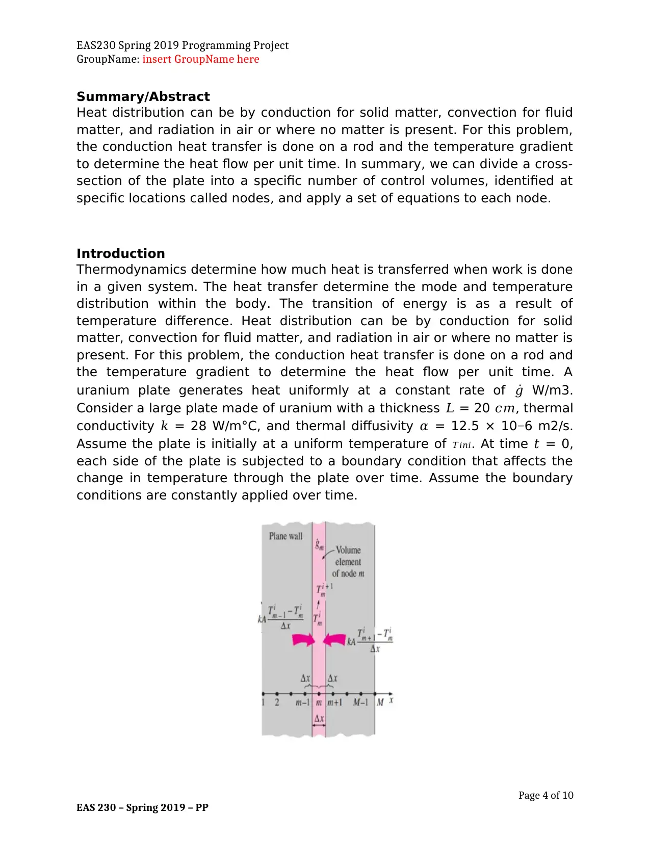
Introduction
Thermodynamics determine how much heat is transferred when work is done
in a given system. The heat transfer determine the mode and temperature
distribution within the body. The transition of energy is as a result of
temperature difference. Heat distribution can be by conduction for solid
matter, convection for fluid matter, and radiation in air or where no matter is
present. For this problem, the conduction heat transfer is done on a rod and
the temperature gradient to determine the heat flow per unit time. A
uranium plate generates heat uniformly at a constant rate of 𝑔̇ W/m3.
Consider a large plate made of uranium with a thickness 𝐿 = 20 𝑐𝑚, thermal
conductivity 𝑘 = 28 W/m°C, and thermal diffusivity 𝛼 = 12.5 × 10⁻⁶ m2/s.
Assume the plate is initially at a uniform temperature of 𝑇𝑖𝑛𝑖. At time 𝑡 = 0,
each side of the plate is subjected to a boundary condition that affects the
change in temperature through the plate over time. Assume the boundary
conditions are constantly applied over time.
Page 4 of 10
EAS 230 – Spring 2019 – PP
GroupName: insert GroupName here
Summary/Abstract
Heat distribution can be by conduction for solid matter, convection for fluid
matter, and radiation in air or where no matter is present. For this problem,
the conduction heat transfer is done on a rod and the temperature gradient
to determine the heat flow per unit time. In summary, we can divide a cross-
section of the plate into a specific number of control volumes, identified at
specific locations called nodes, and apply a set of equations to each node.
Introduction
Thermodynamics determine how much heat is transferred when work is done
in a given system. The heat transfer determine the mode and temperature
distribution within the body. The transition of energy is as a result of
temperature difference. Heat distribution can be by conduction for solid
matter, convection for fluid matter, and radiation in air or where no matter is
present. For this problem, the conduction heat transfer is done on a rod and
the temperature gradient to determine the heat flow per unit time. A
uranium plate generates heat uniformly at a constant rate of 𝑔̇ W/m3.
Consider a large plate made of uranium with a thickness 𝐿 = 20 𝑐𝑚, thermal
conductivity 𝑘 = 28 W/m°C, and thermal diffusivity 𝛼 = 12.5 × 10⁻⁶ m2/s.
Assume the plate is initially at a uniform temperature of 𝑇𝑖𝑛𝑖. At time 𝑡 = 0,
each side of the plate is subjected to a boundary condition that affects the
change in temperature through the plate over time. Assume the boundary
conditions are constantly applied over time.
Page 4 of 10
EAS 230 – Spring 2019 – PP
Paraphrase This Document
Need a fresh take? Get an instant paraphrase of this document with our AI Paraphraser
EAS230 Spring 2019 Programming Project
GroupName: insert GroupName here
Numerical methods are commonly used to determine the changes in temperature
along the thickness of the plate. One such method is called the finite difference
method. In summary, we can divide a cross-section of the plate into a specific
number of control volumes, identified at specific locations called nodes, and apply a
set of equations to each node.
Code
Divide this section into subsections
3.1 Script file
% ------------------------------------------------------------------------%%
% Student Full Name - student personal number - UbitNames
% Lab Sections
% ------------------------------------------------------------------------%%
% Full description of the program and the variables used
% ------------------------------------------------------------------------%%
%% Part 1
L=0; % Plate length
k=0; % Thermal Conductivity
alpha=0; % Thermal Diffusivity
%% Part 2
gbar=input('Enter the Energy Generated within the plate(W/m3):');
M=input('Enter the number of nodes(division in space):');
if(M<2 || ~isinteger(M))
{
disp('Invalid Entry!!!'); %Displays error
M=input('Re-Enter the number of nodes(division in space):');
}
tmax=input('Enter the total time of the simulation (seconds):');
Init_cond=input('Enter initial conditions in form of a vector of M elements of
the temperature profile(at t=0):');
%% printing out the menu showing boundary condition options
fprintf('Boundary Condition for node 1\n 1.For prescribed temperature.\n
2.For prescribed heat flux. \n 3.For insulated. \n 4. For convective.\n');
node1=input('Enter choice number for Node I:')
%using a while loop to validate an entry
tempI=input('Enter the prescribed constant temperature(0C):');
Page 5 of 10
EAS 230 – Spring 2019 – PP
EAS230 Spring 2019 Programming Project
GroupName: insert GroupName here
heat_fluxI=input('Enter the prescribed heat flux(W/m2):');
convectiveI=input('Enter the heat transfer coefficient (W/m2.K):');
temp_outI=input('Enter the outside temperature in 0C:');
%% printing out the menu showing boundary condition options
fprintf('Boundary Condition for node 1\n 1.For prescribed temperature.\n
2.For prescribed heat flux. \n 3.For insulated. \n 4. For convective.\n');
nodeM=input('Enter choice numbers for Node M:')
%using a while loop to validate an entry
tempM=input('Enter the prescribed constant temperature(0C):');
heat_fluxM=input('Enter the prescribed heat flux(W/m2):');
convectiveM=input('Enter the heat transfer coefficient (W/m2.K):');
temp_outM=input('Enter the outside temperature in 0C:');
fprintf('Kindly specify the type of solver.\n 1. Explicit solver. \n 2. Implicit
solver.\n');
solvetype=input('Enter Choice Number of the solver:');
%% Part 3
%calling the explicit solver
explicitsolver();
3.2 Explicit solver
function explicitsolver()
%1 Function parameters
N = 500;
Lx = 50;
dx = Lx/(N-1);
x = 0:dx:Lx;
alpha = .25; % To insure stability alpha = dt/dx^2 < = 1/2
% 2. Time vector
M = 300;
tf = 100;
dt = tf/(M-1);
t = 0:dt:tf;
% 4. Initial and boundary conditions
f = @(x) x; % initial cond. f(x)
g1 = @(t) 1; % boundary conditions g1(t) and g2(t)
g2 = @(t) 1;
% 5. Inilization of the heat equation
u = zeros(N,M);
u(:,1) = f(x);
u(1,:) = g1(t);
% 6. Implementation of the explicit method
for j= 1:M-1 % Time Loop
Page 6 of 10
EAS 230 – Spring 2019 – PP
⊘ This is a preview!⊘
Do you want full access?
Subscribe today to unlock all pages.
Trusted by 1+ million students worldwide
EAS230 Spring 2019 Programming Project
GroupName: insert GroupName here
for i= 2:N-1 % Space Loop
u(i,j+1) = alpha*(u(i-1,j))+(1-2*alpha)*u(i,j) + alpha*u(i+1,j);
end
% Vectorize the inner for loop with this line to gain some speed.
% u(2:N-1,j+1) = alpha*(u(1:N-2,j))+(1-2*alpha)*u(2:N-1,j) +
alpha*u(3:N,j);
% Insert boundary conditions for i = 1 and i = N here.
u(2,j+1) = alpha*u(1,j) + (1-2*alpha)*u(2,j) + alpha*u(3,j);
u(N,j+1) = 2*alpha*u(N-1,j)+(1-2*alpha)*u(N,j)+ 2*alpha*dx*g2(t);
end
% Plot results
figure
plot(x,u(1:end,1:30),'linewidth',2);
a = ylabel('Temperature');
set(a,'Fontsize',14);
a = xlabel('x');
set(a,'Fontsize',14);
a=title(['Using The Explicit Method - alpha =' num2str(alpha)]);
legend('Explicit soln')
set(a,'Fontsize',16);
xlim([0 1]);
grid;
figure
[X, T] = meshgrid(x,t);
s2 = mesh(X',T',u);
title(['3-D plot of the 1D Heat Eq. using the Explicit Method - alpha = '
num2str(alpha)])
set(s2,'FaceColor',[1 0 1],'edgecolor',[0 0 0],'LineStyle','--');
a = title('Explicit finite difference solution of the 1D Diffusivity
Equation');
set(a,'fontsize',14);
a = xlabel('x');
set(a,'fontsize',20);
a = ylabel('y');
set(a,'fontsize',20);
a = zlabel('z');
set(a,'fontsize',20);
xlim([0 2])
zlim([0 2.5])
end
3.3 Implicit solver
Fimp = @(t, x, dx)([dx(1)-x(2); exp(dx(2))+dx(2)+x(1)]);
x0=[1, 0]; dx0=[0,0]; % ICs
F_atx0=[0,exp(0)+1]; F_atdx0=[]; % Function values at x0 and dx0
% Find Consistent Initial values
Page 7 of 10
EAS 230 – Spring 2019 – PP
Paraphrase This Document
Need a fresh take? Get an instant paraphrase of this document with our AI Paraphraser
EAS230 Spring 2019 Programming Project
GroupName: insert GroupName here
[x0, dx0]=decic(Fimp, 0, x0, dx0, F_atx0, F_atdx0);
[t, ft]=ode15i(Fimp, [0,13], x0,dx0);
plot(t, ft(:,1), 'bx-', 'linewidth', 1.5)
hold on
%%
%% Part 2
% Another way of solving this problem is SIMULINK modeling
technique.
% SIMULINK model is executed by the following commands:
load_system('IMPLICIT_2nd_ORDER_ODE.mdl')
set_param('IMPLICIT_2nd_ORDER_ODE','Solver','ode15s','StopTime','13'
);
warning('off');
[t, Y_t]=sim('IMPLICIT_2nd_ORDER_ODE', [0 13]);
plot(t, Y_t(:,1), 'ro--', 'linewidth', 1.5)
legend('ode15i', 'Simulink ode15s')
title(['IMPLICIT 2nd-order ODE problem solved with ODE15i',...
'exp(x")+x"+x=0 with ICs: x(0)=1, dx(0)=0'])
xlabel('t, Time'), ylabel('x(t), Solution')
xlim([0, 13]); grid on; shg
Results
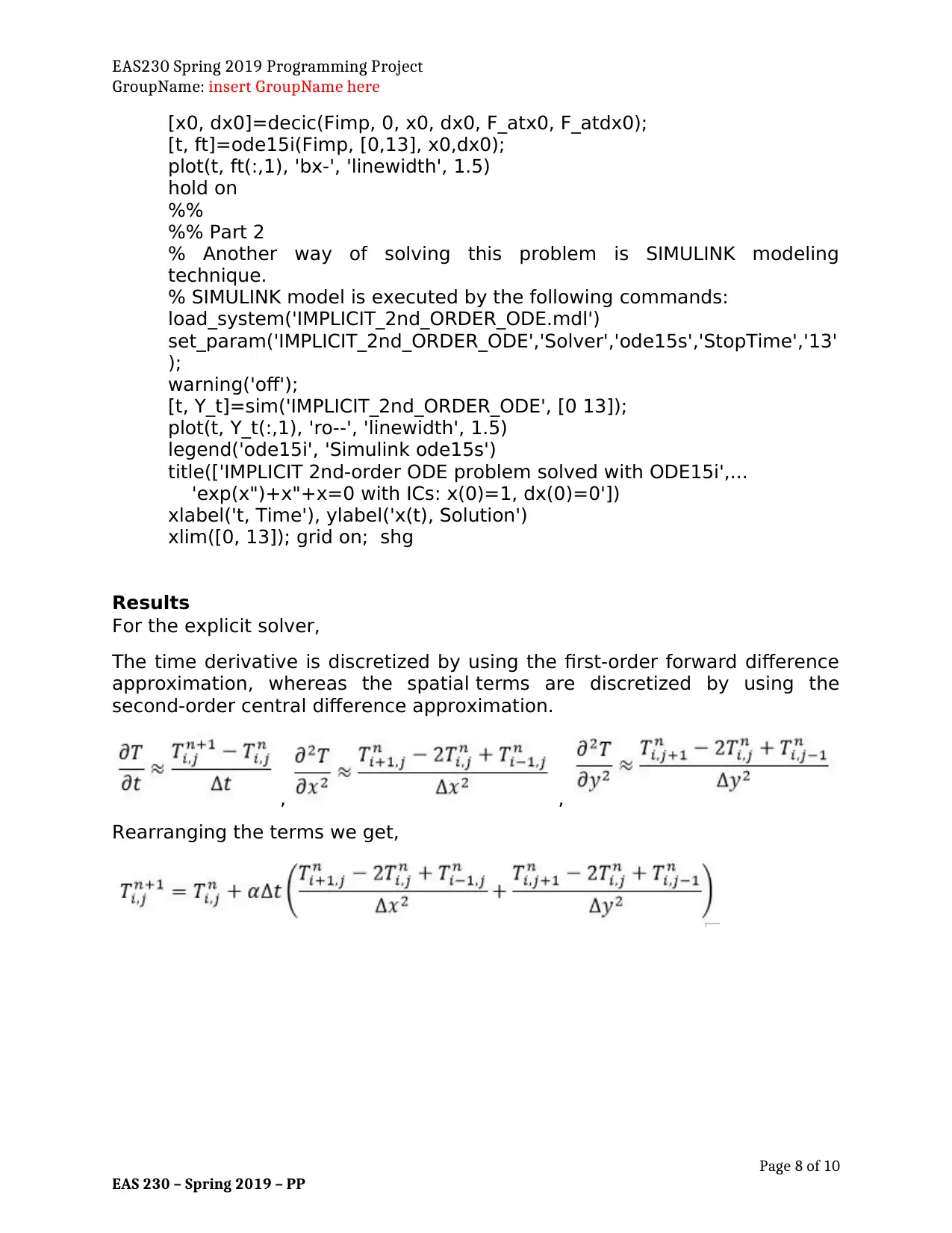
For the explicit solver,
The time derivative is discretized by using the first-order forward difference
approximation, whereas the spatial terms are discretized by using the
second-order central difference approximation.
, ,
Rearranging the terms we get,
Page 8 of 10
EAS 230 – Spring 2019 – PP
GroupName: insert GroupName here
[x0, dx0]=decic(Fimp, 0, x0, dx0, F_atx0, F_atdx0);
[t, ft]=ode15i(Fimp, [0,13], x0,dx0);
plot(t, ft(:,1), 'bx-', 'linewidth', 1.5)
hold on
%%
%% Part 2
% Another way of solving this problem is SIMULINK modeling
technique.
% SIMULINK model is executed by the following commands:
load_system('IMPLICIT_2nd_ORDER_ODE.mdl')
set_param('IMPLICIT_2nd_ORDER_ODE','Solver','ode15s','StopTime','13'
);
warning('off');
[t, Y_t]=sim('IMPLICIT_2nd_ORDER_ODE', [0 13]);
plot(t, Y_t(:,1), 'ro--', 'linewidth', 1.5)
legend('ode15i', 'Simulink ode15s')
title(['IMPLICIT 2nd-order ODE problem solved with ODE15i',...
'exp(x")+x"+x=0 with ICs: x(0)=1, dx(0)=0'])
xlabel('t, Time'), ylabel('x(t), Solution')
xlim([0, 13]); grid on; shg
Results
For the explicit solver,
The time derivative is discretized by using the first-order forward difference
approximation, whereas the spatial terms are discretized by using the
second-order central difference approximation.
, ,
Rearranging the terms we get,
Page 8 of 10
EAS 230 – Spring 2019 – PP
EAS230 Spring 2019 Programming Project
GroupName: insert GroupName here
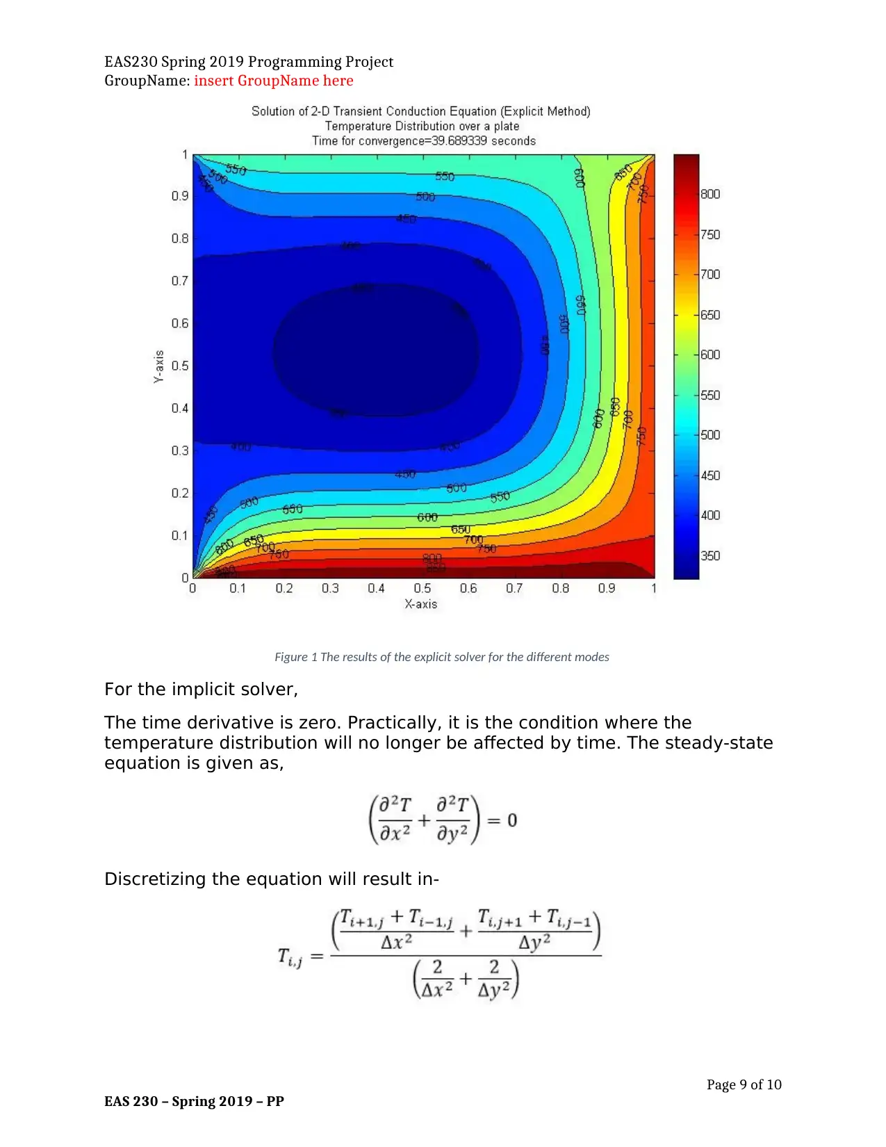
Figure 1 The results of the explicit solver for the different modes
For the implicit solver,
The time derivative is zero. Practically, it is the condition where the
temperature distribution will no longer be affected by time. The steady-state
equation is given as,
Discretizing the equation will result in-
Page 9 of 10
EAS 230 – Spring 2019 – PP
GroupName: insert GroupName here
Figure 1 The results of the explicit solver for the different modes
For the implicit solver,
The time derivative is zero. Practically, it is the condition where the
temperature distribution will no longer be affected by time. The steady-state
equation is given as,
Discretizing the equation will result in-
Page 9 of 10
EAS 230 – Spring 2019 – PP
⊘ This is a preview!⊘
Do you want full access?
Subscribe today to unlock all pages.
Trusted by 1+ million students worldwide
EAS230 Spring 2019 Programming Project
GroupName: insert GroupName here
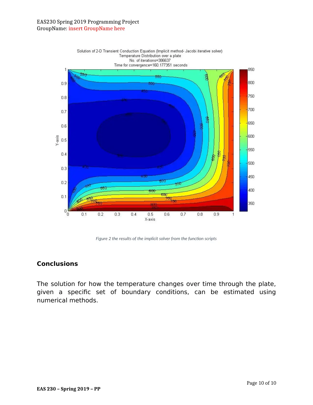
Figure 2 the results of the implicit solver from the function scripts
Conclusions
The solution for how the temperature changes over time through the plate,
given a specific set of boundary conditions, can be estimated using
numerical methods.
Page 10 of 10
EAS 230 – Spring 2019 – PP
GroupName: insert GroupName here
Figure 2 the results of the implicit solver from the function scripts
Conclusions
The solution for how the temperature changes over time through the plate,
given a specific set of boundary conditions, can be estimated using
numerical methods.
Page 10 of 10
EAS 230 – Spring 2019 – PP
1 out of 10

Your All-in-One AI-Powered Toolkit for Academic Success.
+13062052269
info@desklib.com
Available 24*7 on WhatsApp / Email
![[object Object]](/_next/static/media/star-bottom.7253800d.svg)
Unlock your academic potential
Copyright © 2020–2026 A2Z Services. All Rights Reserved. Developed and managed by ZUCOL.