ICT110: Health & Population Data Analysis - East Asia & Pacific
VerifiedAdded on 2023/06/11
|17
|3130
|360
Report
AI Summary
This report provides a comprehensive data analysis of health and population statistics for East Asian and Pacific countries from 2001 to 2015, using data sourced from the World Bank. The analysis includes one-variable and two-variable explorations using boxplots and histograms to understand distributions of unemployment and GNI per capita. Advanced techniques such as k-means clustering are applied to group countries based on GNI and unemployment, while linear regression models explore relationships between health expenditure, GNI, and unemployment rates. The report concludes by summarizing the key findings and reflecting on the analytical process, highlighting the potential use of these insights for policymakers and planners in the region. Desklib provides access to similar reports and solved assignments for students.

Data analysis report of the health and population statistics of East Asian and Pacific countries
Name of the Student
Name of the Student
Paraphrase This Document
Need a fresh take? Get an instant paraphrase of this document with our AI Paraphraser
Table of Contents
1 Introduction..................................................................................................................................1
1.1 Authorisation and Purpose...............................................................................................1
Limitations...................................................................................................................................1
Scope............................................................................................................................................1
Methodology...............................................................................................................................1
2 Data Setup....................................................................................................................................1
3 Exploratory Data Analysis.............................................................................................................2
3.1 One Variable Analysis................................................................................................................2
3.1.1 One Variable Analysis – 1.......................................................................................................2
3.1.2 One Variable Analysis – 2.......................................................................................................3
3.1.3 One Variable Analysis – 3.......................................................................................................5
3.2 Two-variable analysis.................................................................................................................6
3.2.1 Two-variable analysis 1...........................................................................................................6
3.2.2 Two-variable analysis 2...........................................................................................................7
4 Advanced analysis.........................................................................................................................9
4.1 Clustering...................................................................................................................................9
4.1.1 Brief explanation of k-means and clustering..........................................................................9
4.1.2 Clustering Analysis..................................................................................................................9
4.2 Linear regression......................................................................................................................11
4.2.1 Brief definition of linear regression......................................................................................11
4.2.2 Linear Regression 1...............................................................................................................11
4.2.3 Linear Regression 2...............................................................................................................13
5 Conclusion...................................................................................................................................14
6 Reflection....................................................................................................................................14
Reference.......................................................................................................................................16
Page | ii
1 Introduction
1.1 Authorisation and Purpose
The endeavour of the present study is to investigate the health of East Asia and Pacific region.
Information for the period of 2001 to 2015 is taken for the analysis. For the purpose of the
study data has been collected from World Bank. The outcome of the present analysis can be
used by planners, governments to assess the relation of health and various attributes of health
of the region.
Limitations
The facts presented for the analysis pertains to the region of East Asia and Pacific only. Further,
the data pertains to the time period of 2001 to 2015. In addition, information on certain
attributes are missing for some countries.
Scope
The facts for the present analysis consists of 26 attributes concerning health of the region. The
information pertains to East Asia and Pacific region for the period of 2001 to 2015.
The scope of the present study is limited by the presence of missing data. Statistical analysis of
the data is undertaken. Graphs are used to provide a visual representation of the statistical
analysis.
Four different types of graphs are used for the analysis. One-variable and two-variable analysis
are used to represent the attributes. k-means clustering analysis is used to relate the countries
of the region. Linear regression analysis is used to find the relation between attributes.
Methodology
Data collected from World Bank on the health aspects of the East Asia and Pacific region for the
period of 2001 to 2015 is used for the analysis.
2 Data Setup
Prior to starting of the analysis it is important that the data file be imported in “R-program.” In
addition, the “R-program” would require library files for the analysis. Thus the first lines of code
is used for importing the data file into “R.”
The first line also provides information to the “R-program” –
1. The data file to be imported is a CSV file
2. The first row of information is to be taken as header
3. The values are separated by comma
4. There are missing values
⊘ This is a preview!⊘
Do you want full access?
Subscribe today to unlock all pages.
Trusted by 1+ million students worldwide
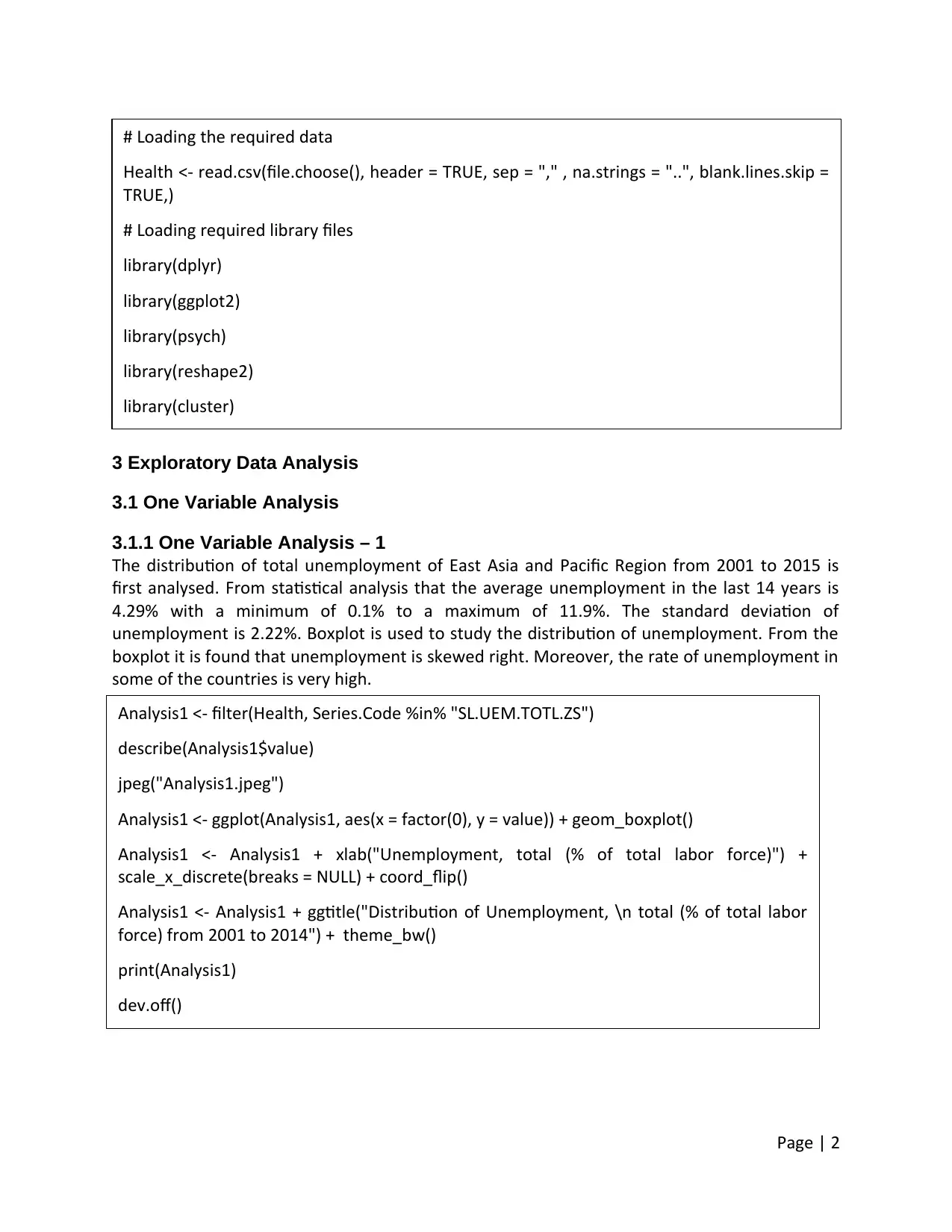
3 Exploratory Data Analysis
3.1 One Variable Analysis
3.1.1 One Variable Analysis – 1
The distribution of total unemployment of East Asia and Pacific Region from 2001 to 2015 is
first analysed. From statistical analysis that the average unemployment in the last 14 years is
4.29% with a minimum of 0.1% to a maximum of 11.9%. The standard deviation of
unemployment is 2.22%. Boxplot is used to study the distribution of unemployment. From the
boxplot it is found that unemployment is skewed right. Moreover, the rate of unemployment in
some of the countries is very high.
Page | 2
Analysis1 <- filter(Health, Series.Code %in% "SL.UEM.TOTL.ZS")
describe(Analysis1$value)
jpeg("Analysis1.jpeg")
Analysis1 <- ggplot(Analysis1, aes(x = factor(0), y = value)) + geom_boxplot()
Analysis1 <- Analysis1 + xlab("Unemployment, total (% of total labor force)") +
scale_x_discrete(breaks = NULL) + coord_flip()
Analysis1 <- Analysis1 + ggtitle("Distribution of Unemployment, \n total (% of total labor
force) from 2001 to 2014") + theme_bw()
print(Analysis1)
dev.off()
# Loading the required data
Health <- read.csv(file.choose(), header = TRUE, sep = "," , na.strings = "..", blank.lines.skip =
TRUE,)
# Loading required library files
library(dplyr)
library(ggplot2)
library(psych)
library(reshape2)
library(cluster)
Paraphrase This Document
Need a fresh take? Get an instant paraphrase of this document with our AI Paraphraser
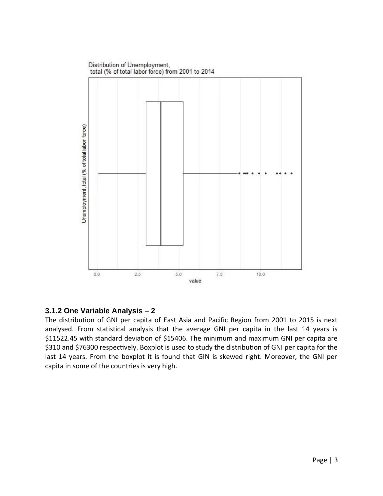
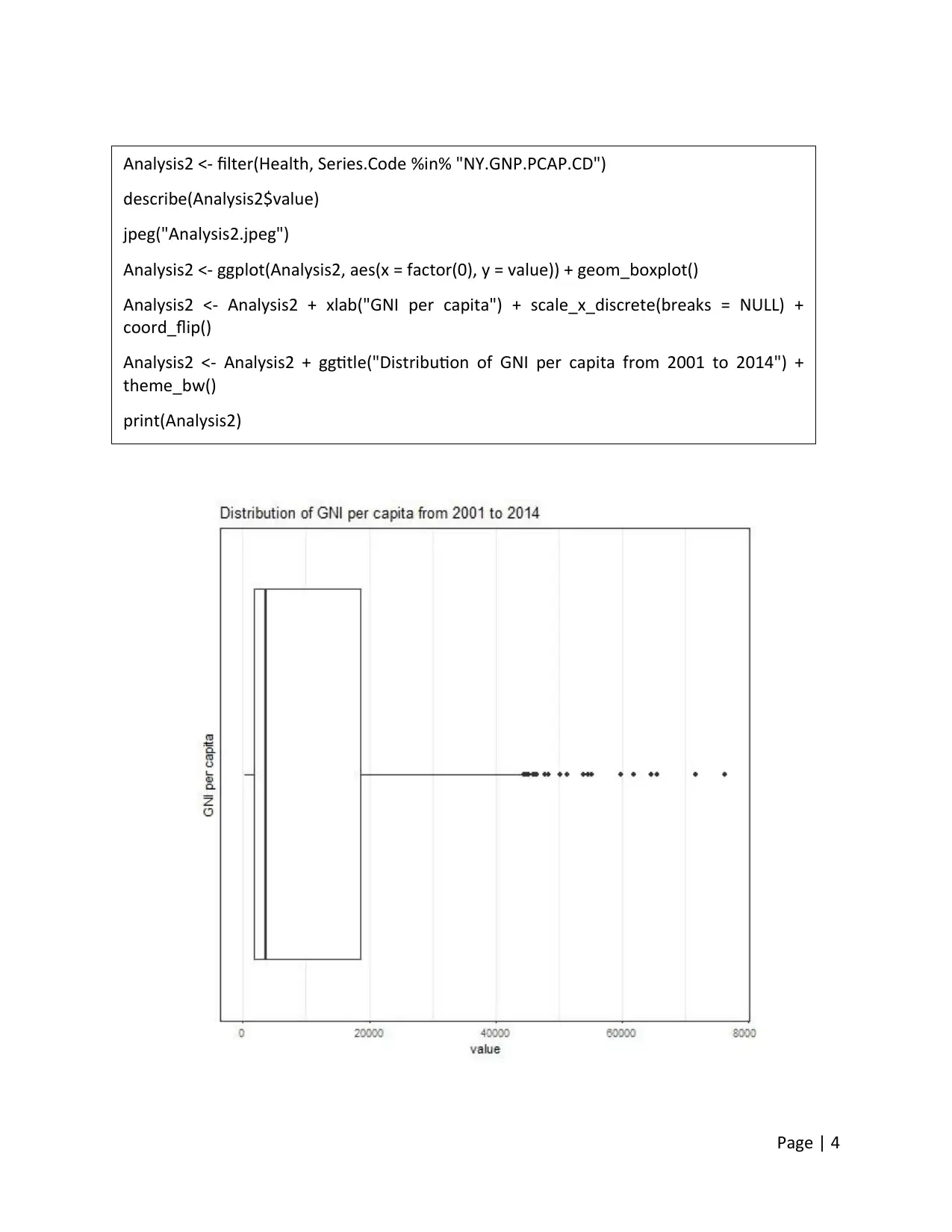
3.1.2 One Variable Analysis – 2
The distribution of GNI per capita of East Asia and Pacific Region from 2001 to 2015 is next
analysed. From statistical analysis that the average GNI per capita in the last 14 years is
$11522.45 with standard deviation of $15406. The minimum and maximum GNI per capita are
$310 and $76300 respectively. Boxplot is used to study the distribution of GNI per capita for the
last 14 years. From the boxplot it is found that GIN is skewed right. Moreover, the GNI per
capita in some of the countries is very high.
Page | 3
Page | 4
Analysis2 <- filter(Health, Series.Code %in% "NY.GNP.PCAP.CD")
describe(Analysis2$value)
jpeg("Analysis2.jpeg")
Analysis2 <- ggplot(Analysis2, aes(x = factor(0), y = value)) + geom_boxplot()
Analysis2 <- Analysis2 + xlab("GNI per capita") + scale_x_discrete(breaks = NULL) +
coord_flip()
Analysis2 <- Analysis2 + ggtitle("Distribution of GNI per capita from 2001 to 2014") +
theme_bw()
print(Analysis2)
⊘ This is a preview!⊘
Do you want full access?
Subscribe today to unlock all pages.
Trusted by 1+ million students worldwide
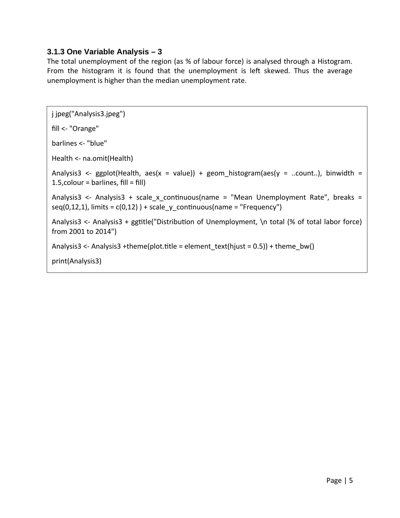
3.1.3 One Variable Analysis – 3
The total unemployment of the region (as % of labour force) is analysed through a Histogram.
From the histogram it is found that the unemployment is left skewed. Thus the average
unemployment is higher than the median unemployment rate.
Page | 5
j jpeg("Analysis3.jpeg")
fill <- "Orange"
barlines <- "blue"
Health <- na.omit(Health)
Analysis3 <- ggplot(Health, aes(x = value)) + geom_histogram(aes(y = ..count..), binwidth =
1.5,colour = barlines, fill = fill)
Analysis3 <- Analysis3 + scale_x_continuous(name = "Mean Unemployment Rate", breaks =
seq(0,12,1), limits = c(0,12) ) + scale_y_continuous(name = "Frequency")
Analysis3 <- Analysis3 + ggtitle("Distribution of Unemployment, \n total (% of total labor force)
from 2001 to 2014")
Analysis3 <- Analysis3 +theme(plot.title = element_text(hjust = 0.5)) + theme_bw()
print(Analysis3)
Paraphrase This Document
Need a fresh take? Get an instant paraphrase of this document with our AI Paraphraser
3.2 Two-variable analysis
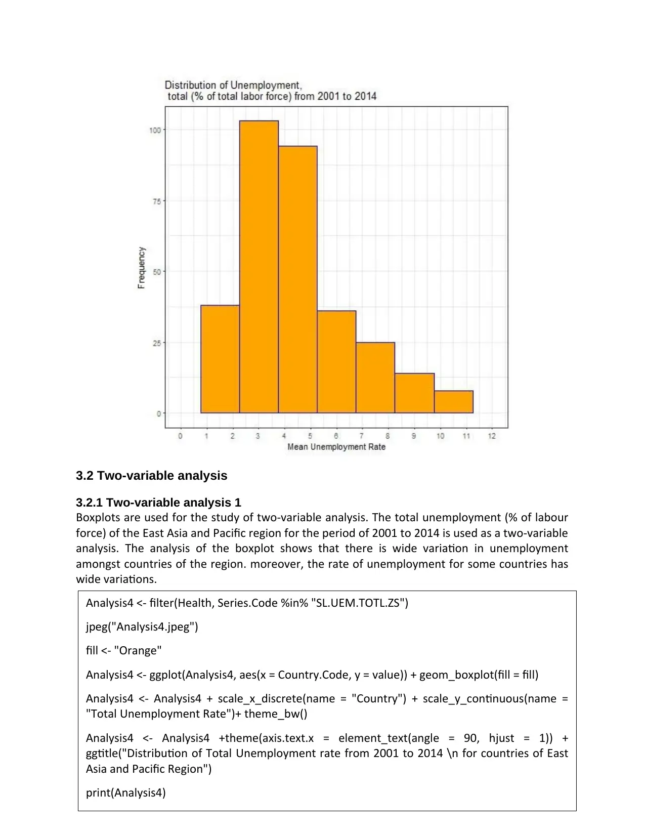
3.2.1 Two-variable analysis 1
Boxplots are used for the study of two-variable analysis. The total unemployment (% of labour
force) of the East Asia and Pacific region for the period of 2001 to 2014 is used as a two-variable
analysis. The analysis of the boxplot shows that there is wide variation in unemployment
amongst countries of the region. moreover, the rate of unemployment for some countries has
wide variations.
Page | 6
Analysis4 <- filter(Health, Series.Code %in% "SL.UEM.TOTL.ZS")
jpeg("Analysis4.jpeg")
fill <- "Orange"
Analysis4 <- ggplot(Analysis4, aes(x = Country.Code, y = value)) + geom_boxplot(fill = fill)
Analysis4 <- Analysis4 + scale_x_discrete(name = "Country") + scale_y_continuous(name =
"Total Unemployment Rate")+ theme_bw()
Analysis4 <- Analysis4 +theme(axis.text.x = element_text(angle = 90, hjust = 1)) +
ggtitle("Distribution of Total Unemployment rate from 2001 to 2014 \n for countries of East
Asia and Pacific Region")
print(Analysis4)
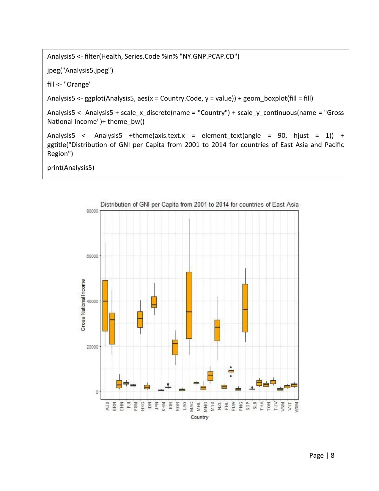
3.2.2 Two-variable analysis 2
Boxplot is used to study the relation GNI per capita of the countries for the period from 2001 to
2014. The use of Boxplot offers the advantage that individual countries of the region can be
compared on the basis of the distribuion of their GNI for the 14 years of study. From the
Boxplot it is found that for most of the countries of the region GNI is less than $10000. For
countries with GNI above $10000 there are wide variations in values for the last 14 years.
Page | 7
⊘ This is a preview!⊘
Do you want full access?
Subscribe today to unlock all pages.
Trusted by 1+ million students worldwide
Page | 8
Analysis5 <- filter(Health, Series.Code %in% "NY.GNP.PCAP.CD")
jpeg("Analysis5.jpeg")
fill <- "Orange"
Analysis5 <- ggplot(Analysis5, aes(x = Country.Code, y = value)) + geom_boxplot(fill = fill)
Analysis5 <- Analysis5 + scale_x_discrete(name = "Country") + scale_y_continuous(name = "Gross
National Income")+ theme_bw()
Analysis5 <- Analysis5 +theme(axis.text.x = element_text(angle = 90, hjust = 1)) +
ggtitle("Distribution of GNI per Capita from 2001 to 2014 for countries of East Asia and Pacific
Region")
print(Analysis5)
Paraphrase This Document
Need a fresh take? Get an instant paraphrase of this document with our AI Paraphraser
4 Advanced analysis
4.1 Clustering
4.1.1 Brief explanation of k-means and clustering
The method of segregating a data into analogous groups is known as clustering. The behaviour
of analogous groups is similar. Clustering involves dividing the data set into groups and thus
allocating data points to such groups (Oleiwi 2016). Data points in a group have similar
properties.
In k-means clustering the data values are segregated into k-groups. In k-means clustering first k-
centroids are identified. Each data is sequentially added to a centroid nearest to its value. When
a second data point is added the centroid is adjusted based on the mean of the two points. This
process is continued until all data points are exhausted (Witten et al., 2016).
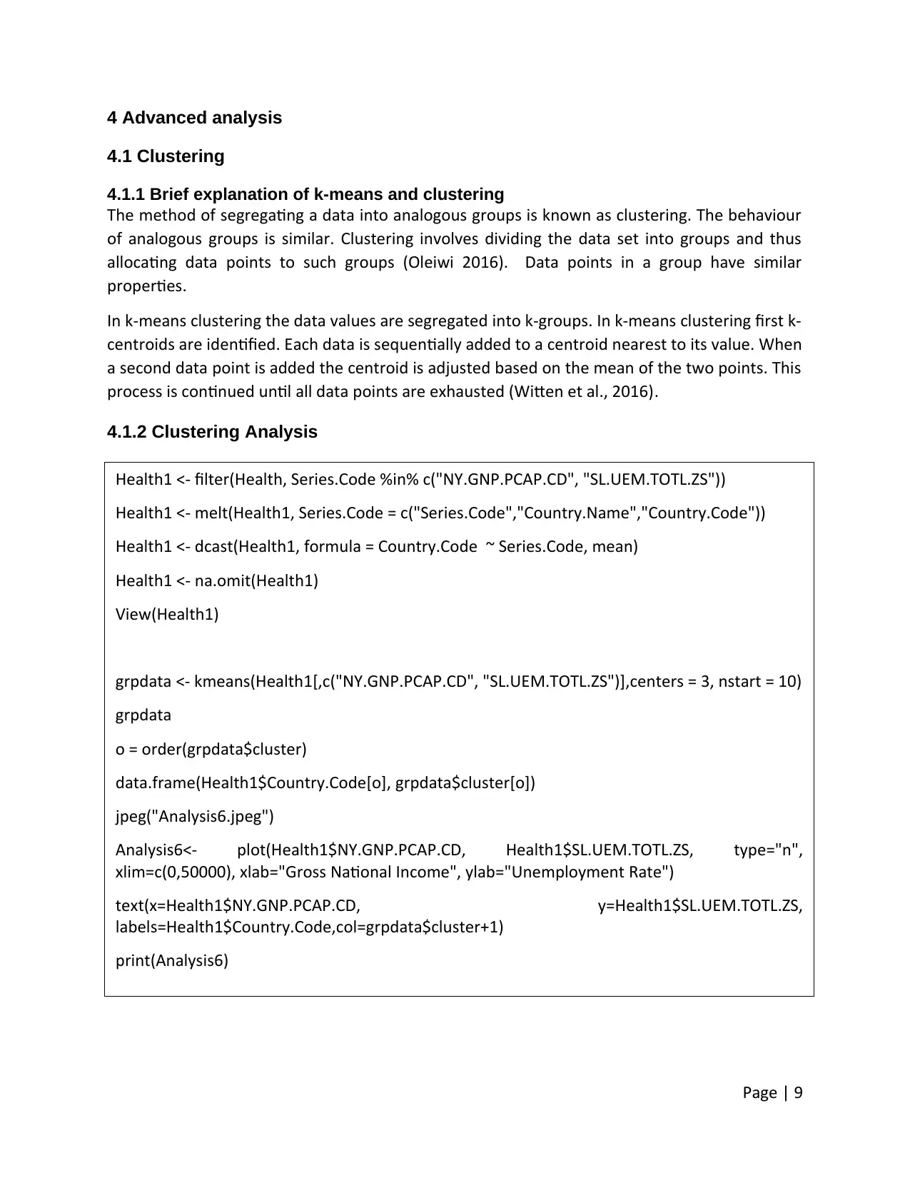
4.1.2 Clustering Analysis
Page | 9
Health1 <- filter(Health, Series.Code %in% c("NY.GNP.PCAP.CD", "SL.UEM.TOTL.ZS"))
Health1 <- melt(Health1, Series.Code = c("Series.Code","Country.Name","Country.Code"))
Health1 <- dcast(Health1, formula = Country.Code ~ Series.Code, mean)
Health1 <- na.omit(Health1)
View(Health1)
grpdata <- kmeans(Health1[,c("NY.GNP.PCAP.CD", "SL.UEM.TOTL.ZS")],centers = 3, nstart = 10)
grpdata
o = order(grpdata$cluster)
data.frame(Health1$Country.Code[o], grpdata$cluster[o])
jpeg("Analysis6.jpeg")
Analysis6<- plot(Health1$NY.GNP.PCAP.CD, Health1$SL.UEM.TOTL.ZS, type="n",
xlim=c(0,50000), xlab="Gross National Income", ylab="Unemployment Rate")
text(x=Health1$NY.GNP.PCAP.CD, y=Health1$SL.UEM.TOTL.ZS,
labels=Health1$Country.Code,col=grpdata$cluster+1)
print(Analysis6)
4.1 Clustering
4.1.1 Brief explanation of k-means and clustering
The method of segregating a data into analogous groups is known as clustering. The behaviour
of analogous groups is similar. Clustering involves dividing the data set into groups and thus
allocating data points to such groups (Oleiwi 2016). Data points in a group have similar
properties.
In k-means clustering the data values are segregated into k-groups. In k-means clustering first k-
centroids are identified. Each data is sequentially added to a centroid nearest to its value. When
a second data point is added the centroid is adjusted based on the mean of the two points. This
process is continued until all data points are exhausted (Witten et al., 2016).
4.1.2 Clustering Analysis
Page | 9
Health1 <- filter(Health, Series.Code %in% c("NY.GNP.PCAP.CD", "SL.UEM.TOTL.ZS"))
Health1 <- melt(Health1, Series.Code = c("Series.Code","Country.Name","Country.Code"))
Health1 <- dcast(Health1, formula = Country.Code ~ Series.Code, mean)
Health1 <- na.omit(Health1)
View(Health1)
grpdata <- kmeans(Health1[,c("NY.GNP.PCAP.CD", "SL.UEM.TOTL.ZS")],centers = 3, nstart = 10)
grpdata
o = order(grpdata$cluster)
data.frame(Health1$Country.Code[o], grpdata$cluster[o])
jpeg("Analysis6.jpeg")
Analysis6<- plot(Health1$NY.GNP.PCAP.CD, Health1$SL.UEM.TOTL.ZS, type="n",
xlim=c(0,50000), xlab="Gross National Income", ylab="Unemployment Rate")
text(x=Health1$NY.GNP.PCAP.CD, y=Health1$SL.UEM.TOTL.ZS,
labels=Health1$Country.Code,col=grpdata$cluster+1)
print(Analysis6)
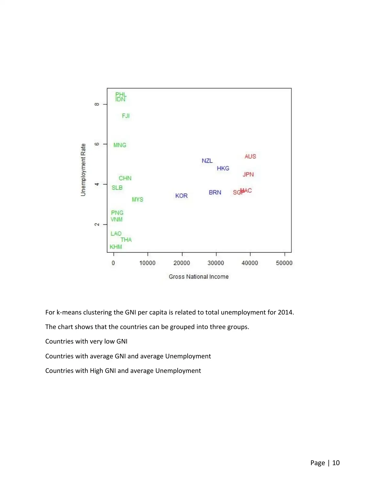
For k-means clustering the GNI per capita is related to total unemployment for 2014.
The chart shows that the countries can be grouped into three groups.
Countries with very low GNI
Countries with average GNI and average Unemployment
Countries with High GNI and average Unemployment
Page | 10
The chart shows that the countries can be grouped into three groups.
Countries with very low GNI
Countries with average GNI and average Unemployment
Countries with High GNI and average Unemployment
Page | 10
⊘ This is a preview!⊘
Do you want full access?
Subscribe today to unlock all pages.
Trusted by 1+ million students worldwide
1 out of 17
Related Documents


Your All-in-One AI-Powered Toolkit for Academic Success.
+13062052269
info@desklib.com
Available 24*7 on WhatsApp / Email
![[object Object]](/_next/static/media/star-bottom.7253800d.svg)
Unlock your academic potential
Copyright © 2020–2026 A2Z Services. All Rights Reserved. Developed and managed by ZUCOL.