Oregon State University ECE 351 Computing Assignment 2 Solutions

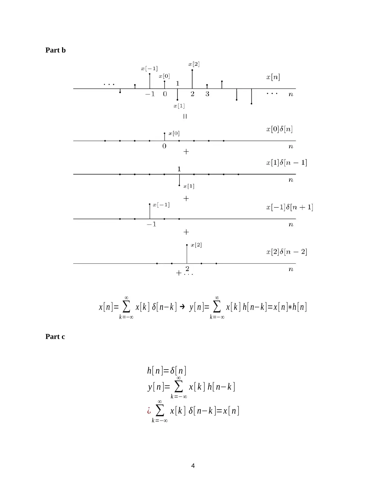
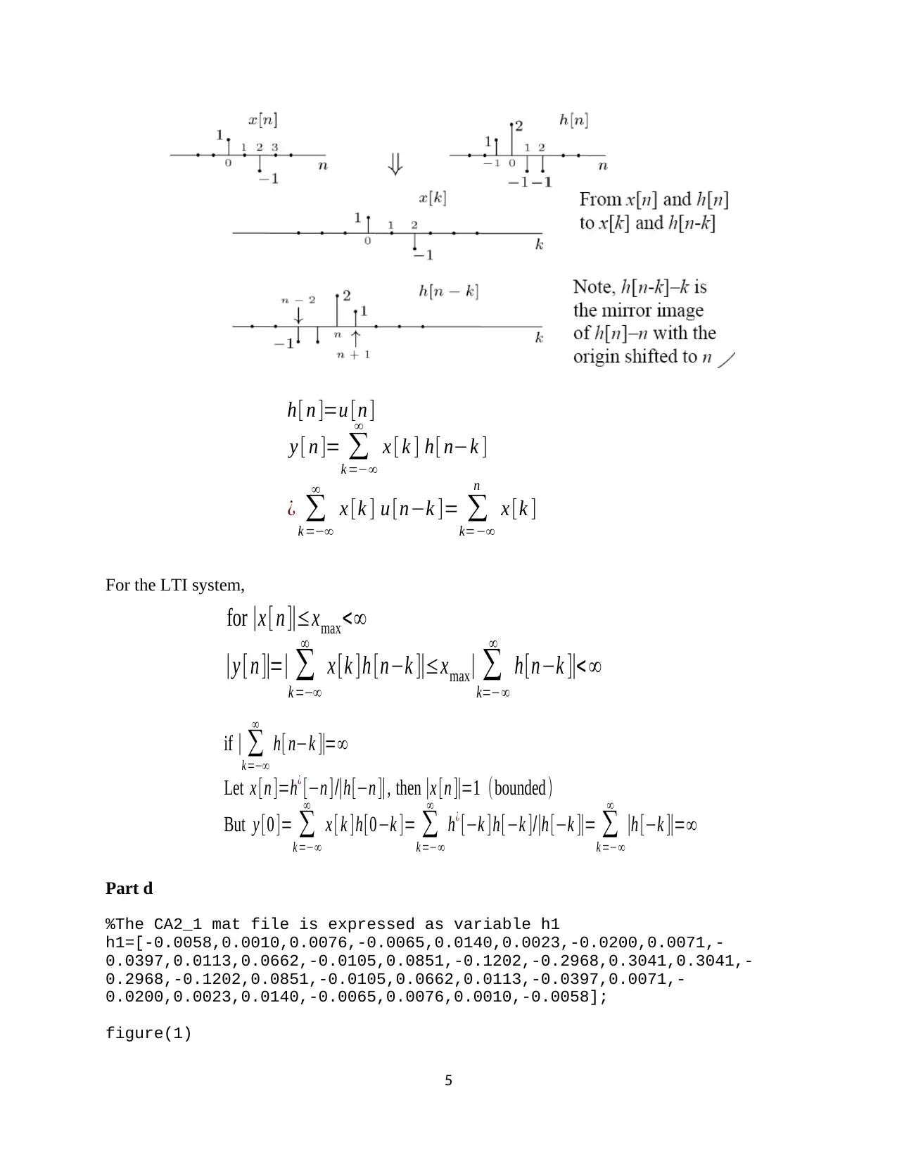
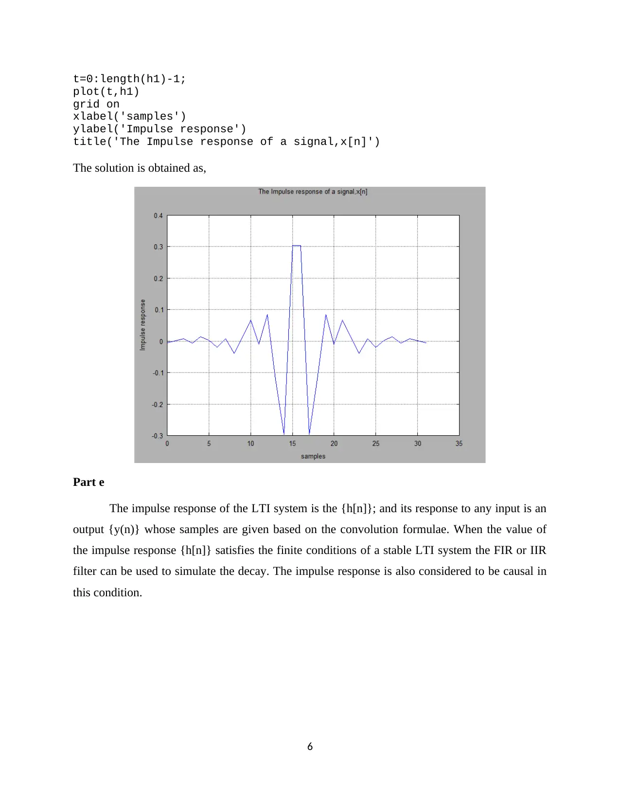
This document presents the complete solution to Computing Assignment 2 for ECE 351 Signals and Systems I at Oregon State University. The assignment explores key concepts in discrete-time signal processing, including normalized frequency and its periodicity, as demonstrated through cosine wave analysis. The solution delves into the properties of Linear Time-Invariant (LTI) systems, impulse responses, and filter design, specifically using Finite Impulse Response (FIR) filters. Question 2 presents a function my_fir, which applies a filter to an input signal. The document also examines the relationship between the impulse response and system stability, and analyzes the practical application of FIR filters in simulating signal decay. MATLAB code and plots are provided to illustrate the concepts, offering a comprehensive understanding of the assignment's requirements.

OREGON STATE UNIVERSITY
SIGNALS AND SYSTEMS I
ECE 351
COMPUTING ASSIGNMENT #2

QUESTION I
The normalized frequency is periodic with a period 2pi rads/sample.
cos ( Ω0 n )=cos ( ( Ω0 +2 πk ) n )
%% SECTION I
%part a
d=rad2deg(pi); %Angle in degrees
W0=d/3; %value in the range of [-180,180]
n=-0.5:0.01:0.5; %range of samples used in the signal analysis
k=5; %for any integer value of k=0,1,2,3...
x1=cos(W0.*n); %signal 1
x2=cos((W0+2*d*k).*n); %signal 2
%part b
figure(1)
plot(n,x1,'r');
grid on
xlabel('Samples')
ylabel('Signal x(n)')
hold on
plot(n,x2,'b');
grid on
hold off
title('Plot of Two Cosine waves: x1(n) & x2(n)');
%part c
%When the signal is obtained as a sampled continuous time sinusoid
t=-5:0.1:5;
wo=1/t; %frequency in radians/sample
T=25; %Sampling frequency
xn=cos((wo*T).*n); %sampled continuous time signal
figure(2)
plot(n,xn);
grid on
xlabel('Frequency(radians/sample)')
ylabel('Signal---x(n)')
title('Sampled Continuous Time signal')
The solution is obtained as,
1

2

QUESTION 2
%% SECTION II
function[y]=my_fir(x,h)
%The function my_fir has input arguments x and h
h = h(:)'; % The vector h is transposed
L = length(h); %The value of L is assigned to the number of values
stored in h
L1 = L-1; %Value L1=L-1
x = [x(:); zeros(L1,1)]; %x is a two row matrix with x vector as row 1
and zeros(L1,1) vector as row 2
y = zeros(size(x));
X = zeros(L,1);
for i = 1:length(x) %The for loop iterates up to the length(x) times
X = [x(i);X(1:L1)];
y(i) = h*X; %The output matrix or vector is generated from the product
h*X
end
The filter used is based on an array or row vector x and y using the recursive difference equation.
QUESTION 3
Part a
3
δ [ n−n0 ]

Part b
Part c
4
x [n ]= ∑
k =−∞
∞
x [k ] δ[ n−k ] → y [ n ]= ∑
k =−∞
∞
x [ k ] h[ n−k ]=x [ n ]∗h [n ]
h[ n ]=δ[ n ]
y [ n ]= ∑
k =−∞
∞
x [ k ] h[ n−k ]
¿ ∑
k =−∞
∞
x [k ] δ[ n−k ]=x [ n ]

For the LTI system,
Part d
%The CA2_1 mat file is expressed as variable h1
h1=[-0.0058,0.0010,0.0076,-0.0065,0.0140,0.0023,-0.0200,0.0071,-
0.0397,0.0113,0.0662,-0.0105,0.0851,-0.1202,-0.2968,0.3041,0.3041,-
0.2968,-0.1202,0.0851,-0.0105,0.0662,0.0113,-0.0397,0.0071,-
0.0200,0.0023,0.0140,-0.0065,0.0076,0.0010,-0.0058];
figure(1)
5
h[ n ]=u [n ]
y [ n ]= ∑
k =−∞
∞
x [ k ] h[ n−k ]
¿ ∑
k =−∞
∞
x [k ] u [n−k ]= ∑
k=−∞
n
x [k ]
for |x [ n ]|≤xmax<∞
|y [ n ]|=| ∑
k =−∞
∞
x [k ]h [n−k ]|≤xmax| ∑
k=−∞
∞
h[n−k ]|< ∞
if | ∑
k =−∞
∞
h[ n−k ]|=∞
Let x [n ]=h¿ [−n ]/|h[−n ]|, then |x [n ]|=1 ( bounded )
But y [0 ]= ∑
k =−∞
∞
x [ k ]h[0−k ]= ∑
k =−∞
∞
h¿ [−k ]h[−k ]/|h [−k ]|= ∑
k =−∞
∞
|h [−k ]|=∞

t=0:length(h1)-1;
plot(t,h1)
grid on
xlabel('samples')
ylabel('Impulse response')
title('The Impulse response of a signal,x[n]')
The solution is obtained as,
Part e
The impulse response of the LTI system is the {h[n]}; and its response to any input is an
output {y(n)} whose samples are given based on the convolution formulae. When the value of
the impulse response {h[n]} satisfies the finite conditions of a stable LTI system the FIR or IIR
filter can be used to simulate the decay. The impulse response is also considered to be causal in
this condition.
6