ECO101 Microeconomics Assignment: Production, Supply & Demand Analysis

This ECO101 microeconomics assignment explores core concepts including production possibility curves, comparative advantage, and supply and demand analysis. It includes calculations and graphical representations to illustrate these principles. The assignment addresses questions related to production efficiency, market equilibrium, and price elasticity of demand. Specific scenarios involving coffee and nut production are analyzed to demonstrate comparative advantage and optimal resource allocation. Additionally, the assignment examines the impact of shifts in supply on market prices within a perfectly competitive market. The document provides detailed solutions and explanations, offering a comprehensive overview of these microeconomic topics.

Unit: ECO101 Microeconomics
1

Question-1
Part-a. Given that Jara can pick 4 kilograms of coffee in an hour or 2 kilograms of
nuts. Peng can pick 2 kilograms of coffee in an hour or 4 kilograms of nuts. Each
works 6 hours per day.
(i) Maximum coffee that Jara can pick in a day = (4)(6) = 24 Kg.Maximum Coffee that
Peng can pick in a day = (2)(6) = 12 kg.Maximum coffeethat can be picked in a day
by both Jara and Peng = 24+12 = 36 Kg.
(ii) Maximum nuts that Jara can pick in a day = (2)(6) = 12 kg. Maximum nuts that Peng
can pick in a day = (4)(6) = 24 kg. Maximum nuts that can be picked in a day by both
Jara and Peng = 12+24 = 36 Kg.
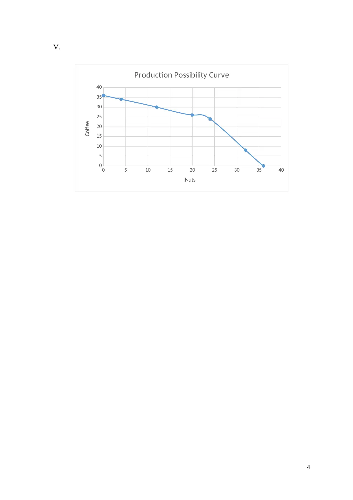
(iii) Since Peng has comparative advantage in picking nuts he will pick 4
kilograms of nuts in 1 hour. Time left to Peng is 5 hours and he will pick coffee
amounting to (5)(2) = 10 kg. Time available to Jara is 6 hours and he will pick Coffee
amounting to (6)(4) = 24 kg. Total nuts picked by Peng 4 Kg. Total coffee picked by
Jara and Peng = 10+24 = 34 Kg.
(iv)Since Jara has comparative advantage in picking coffee, he would pick 8 kg coffees in
2 hours. Time left to Jara 4 hours. In 4 hours he will pick 8 kg of nuts. Peng will pick
(6) (4) = 24 kg of nuts. So Jara would pick up the coffee as he possesses comparative
advantage and both Jaraand Peng will pick nuts amounting to 32 Kg (8 kg by Jara and
24 kg by Peng)
(v) Yes. The above –mentioned situation is feasible ifPeng picks 24 kg nuts in 6 hours
and Jara picks 2 kg nuts in 1 hour. This will make total of 26kg nuts to be picked by
Peng and Jara together. Thereafter Jara would have 5 hours which will be used in
2

picking 20 kg of coffee. So, it is possible to pick 26 kilograms of nuts and 20
kilograms of coffee by both Jara and Peng in total hours allotted to them in a day.
Part-b
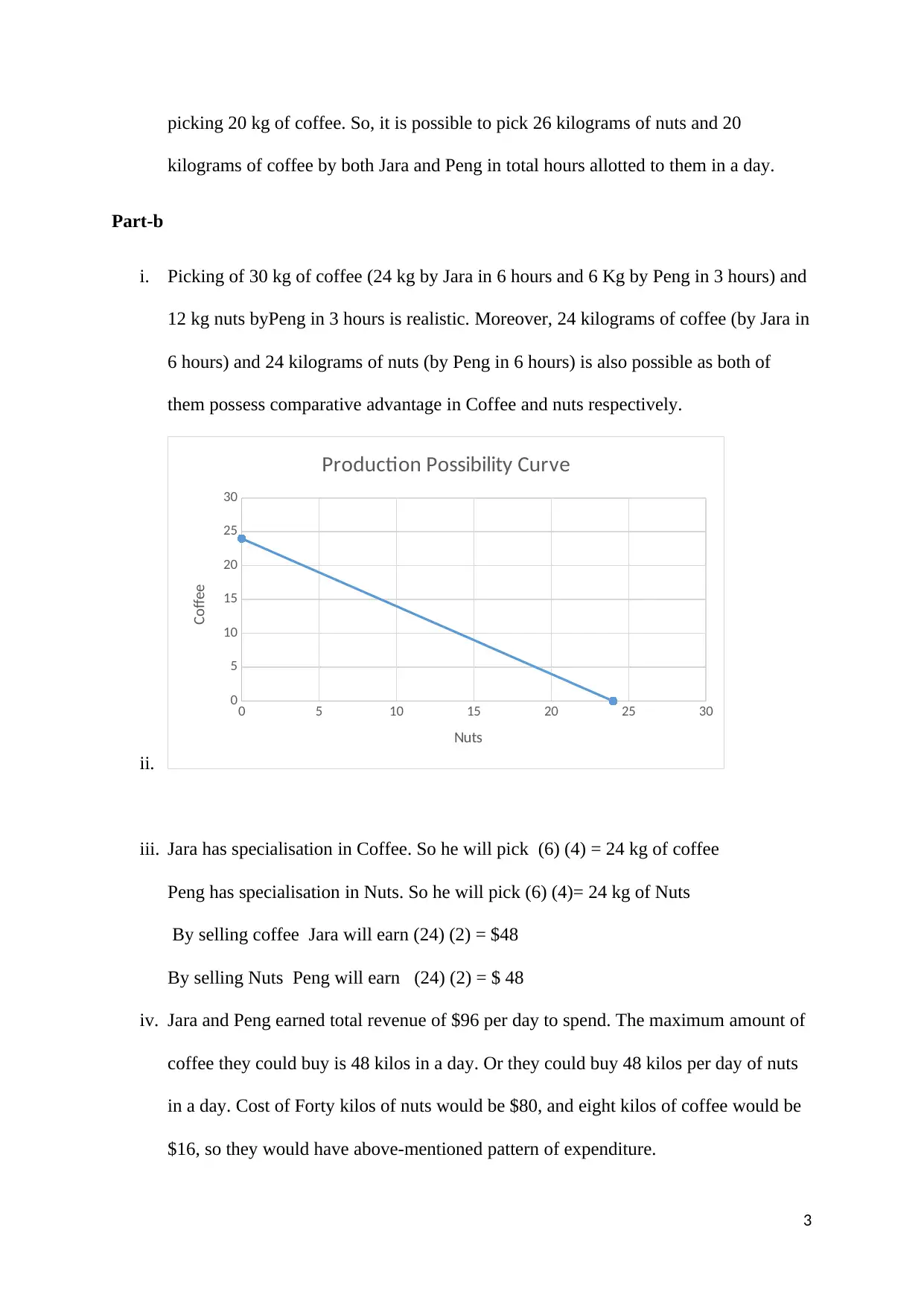
i. Picking of 30 kg of coffee (24 kg by Jara in 6 hours and 6 Kg by Peng in 3 hours) and
12 kg nuts byPeng in 3 hours is realistic. Moreover, 24 kilograms of coffee (by Jara in
6 hours) and 24 kilograms of nuts (by Peng in 6 hours) is also possible as both of
them possess comparative advantage in Coffee and nuts respectively.
ii.
0 5 10 15 20 25 30
0
5
10
15
20
25
30
Production Possibility Curve
Nuts
Coffee
iii. Jara has specialisation in Coffee. So he will pick (6) (4) = 24 kg of coffee
Peng has specialisation in Nuts. So he will pick (6) (4)= 24 kg of Nuts
By selling coffee Jara will earn (24) (2) = $48
By selling Nuts Peng will earn (24) (2) = $ 48
iv. Jara and Peng earned total revenue of $96 per day to spend. The maximum amount of
coffee they could buy is 48 kilos in a day. Or they could buy 48 kilos per day of nuts
in a day. Cost of Forty kilos of nuts would be $80, and eight kilos of coffee would be
$16, so they would have above-mentioned pattern of expenditure.
3

V.
0 5 10 15 20 25 30 35 40
0
5
10
15
20
25
30
35
40
Production Possibility Curve
Nuts
Coffee
4

Question-2
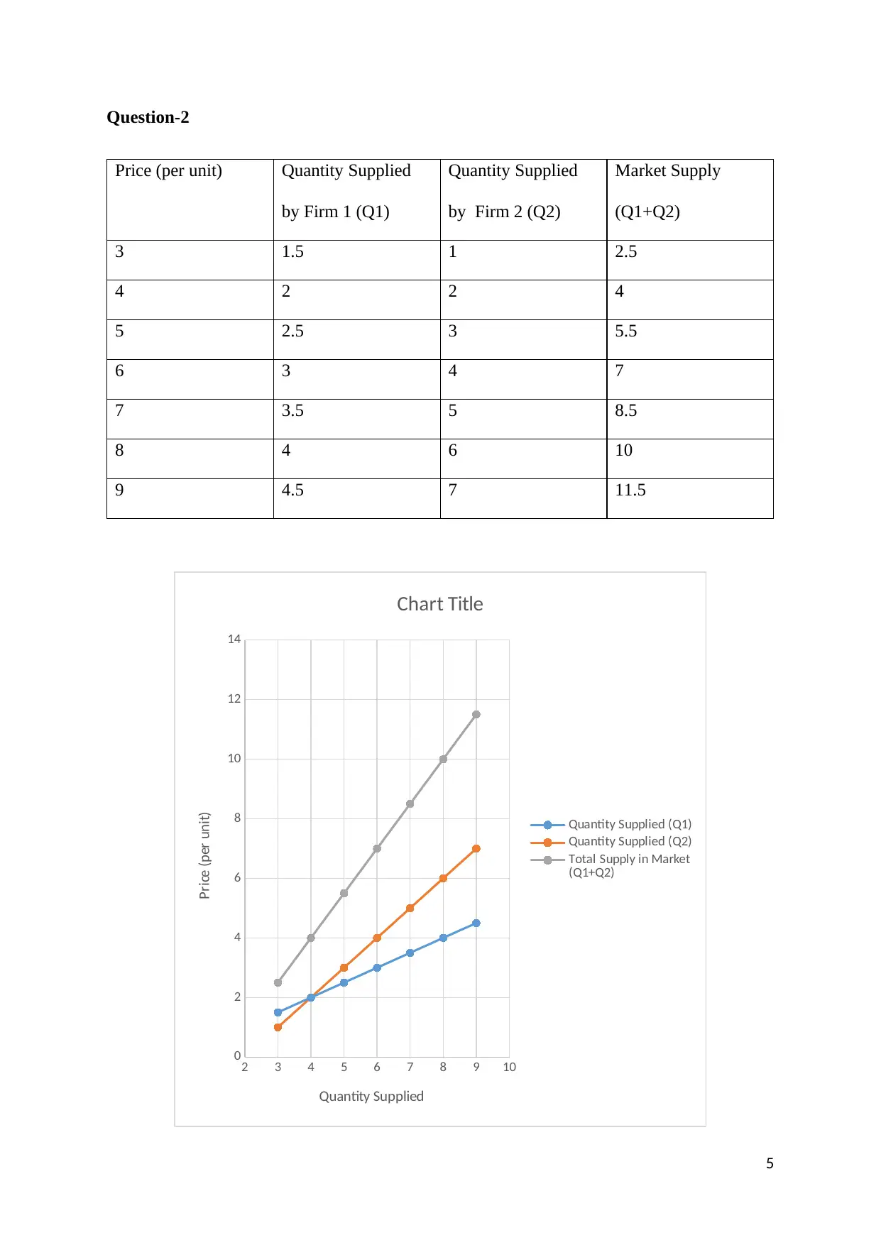
Price (per unit) Quantity Supplied
by Firm 1 (Q1)
Quantity Supplied
by Firm 2 (Q2)
Market Supply
(Q1+Q2)
3 1.5 1 2.5
4 2 2 4
5 2.5 3 5.5
6 3 4 7
7 3.5 5 8.5
8 4 6 10
9 4.5 7 11.5
2 3 4 5 6 7 8 9 10
0
2
4
6
8
10
12
14
Chart Title
Quantity Supplied (Q1)
Quantity Supplied (Q2)
Total Supply in Market
(Q1+Q2)
Quantity Supplied
Price (per unit)
5

Question-3
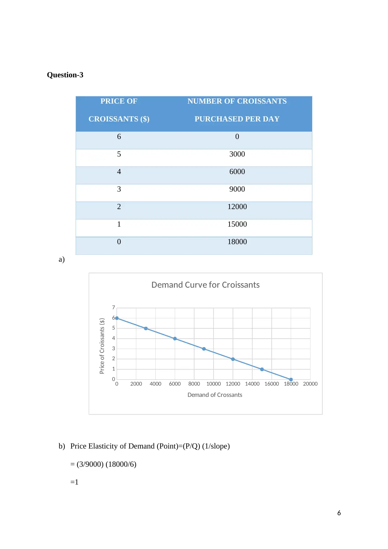
PRICE OF
CROISSANTS ($)
NUMBER OF CROISSANTS
PURCHASED PER DAY
6 0
5 3000
4 6000
3 9000
2 12000
1 15000
0 18000
a)
0 2000 4000 6000 8000 10000 12000 14000 16000 18000 20000
0
1
2
3
4
5
6
7
Demand Curve for Croissants
Demand of Crossants
Price of Croissants ($)
b) Price Elasticity of Demand (Point)=(P/Q) (1/slope)
= (3/9000) (18000/6)
=1
6

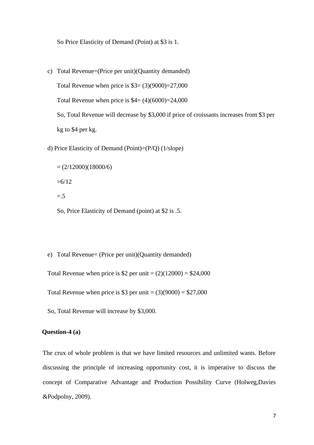
So Price Elasticity of Demand (Point) at $3 is 1.
c) Total Revenue=(Price per unit)(Quantity demanded)
Total Revenue when price is $3= (3)(9000)=27,000
Total Revenue when price is $4= (4)(6000)=24,000
So, Total Revenue will decrease by $3,000 if price of croissants increases from $3 per
kg to $4 per kg.
d) Price Elasticity of Demand (Point)=(P/Q) (1/slope)
= (2/12000)(18000/6)
=6/12
=.5
So, Price Elasticity of Demand (point) at $2 is .5.
e) Total Revenue= (Price per unit)(Quantity demanded)
Total Revenue when price is $2 per unit = (2)(12000) = $24,000
Total Revenue when price is $3 per unit = (3)(9000) = $27,000
So, Total Revenue will increase by $3,000.
Question-4 (a)
The crux of whole problem is that we have limited resources and unlimited wants. Before
discussing the principle of increasing opportunity cost, it is imperative to discuss the
concept of Comparative Advantage and Production Possibility Curve (Holweg,Davies
&Podpolny, 2009).
7

Comparative advantage simply means that a economy can produces a good or service for a
lower opportunity cost than other economies. Opportunity cost is the cost of next best
alternative forgone. An economy with a comparative advantage is not necessarily best in
producing something. The advantages of buying the good or service of that economy
outweigh the disadvantages. This indicates the good or service has a low opportunity cost
for other economies to import.
For instance, countries of Middle East have a comparative advantage in manufacturing
chemicals. Reason being oil is produced in these countries and so oil provides a cheap input
for the chemicals when compared to producing chemicals in other countries.
0 0.5 1 1.5 2 2.5 3 3.5 4 4.5
0
5
10
15
20
25
30
35A B
c
D
E
Production Possibility Curve
Butter
Drainpipe
A B C D E
Butter 0 1 2 3 4
8

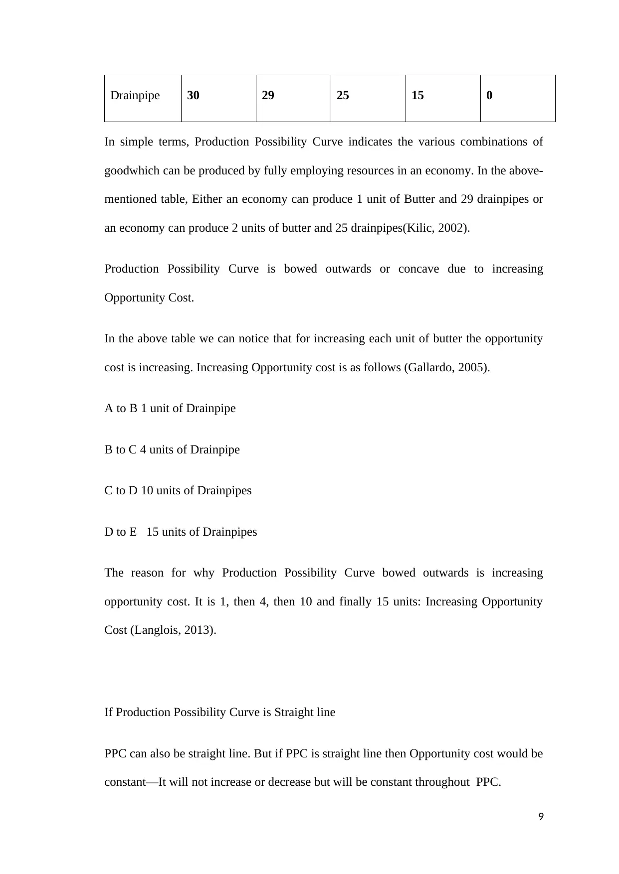
Drainpipe 30 29 25 15 0
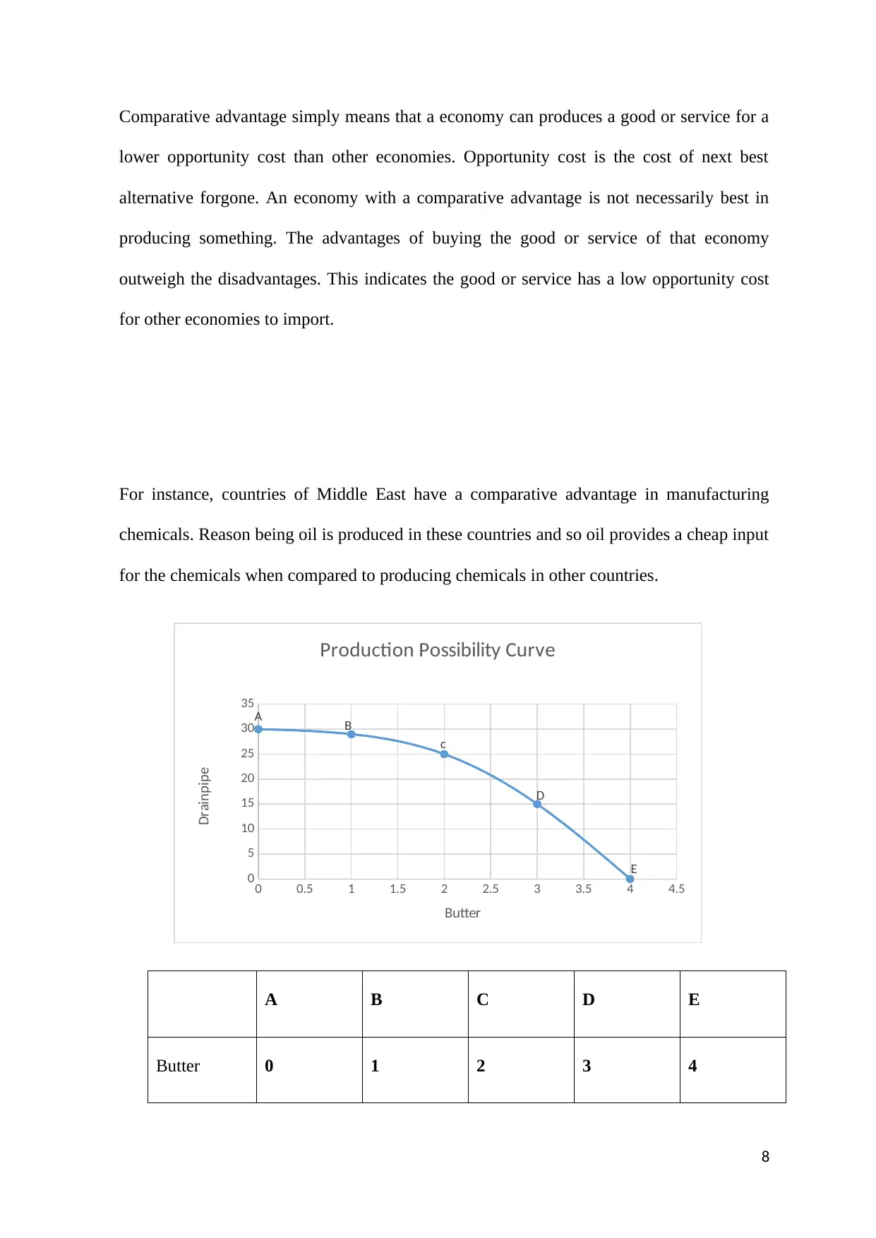
In simple terms, Production Possibility Curve indicates the various combinations of
goodwhich can be produced by fully employing resources in an economy. In the above-
mentioned table, Either an economy can produce 1 unit of Butter and 29 drainpipes or
an economy can produce 2 units of butter and 25 drainpipes(Kilic, 2002).
Production Possibility Curve is bowed outwards or concave due to increasing
Opportunity Cost.
In the above table we can notice that for increasing each unit of butter the opportunity
cost is increasing. Increasing Opportunity cost is as follows (Gallardo, 2005).
A to B 1 unit of Drainpipe
B to C 4 units of Drainpipe
C to D 10 units of Drainpipes
D to E 15 units of Drainpipes
The reason for why Production Possibility Curve bowed outwards is increasing
opportunity cost. It is 1, then 4, then 10 and finally 15 units: Increasing Opportunity
Cost (Langlois, 2013).
If Production Possibility Curve is Straight line
PPC can also be straight line. But if PPC is straight line then Opportunity cost would be
constant—It will not increase or decrease but will be constant throughout PPC.
9

Question-4 (b)
First of all it is important to distinguish between long run and short run. There are
four factors of production: Land, Labour, Capital and Entrepreneurship.The basic
difference between short run and long run is that there are both fixed and variable
factors in the short run. However, in long run all factors are variable. In other words,
there are no fixed factors in the long run and all factors are variable.In the long run, a
firm is free to increase or decrease all of its inputs: land, Labour, Capital and
Entrepreneurship. Existing firms can leave the market and new firms can enter the
market (Holweg,Davies &Podpolny, 2009).
[Source: https://saylordotorg.github.io/text_principles-of-economics-v2.0/s12-03-perfect-
competition-in-the-lon.html]
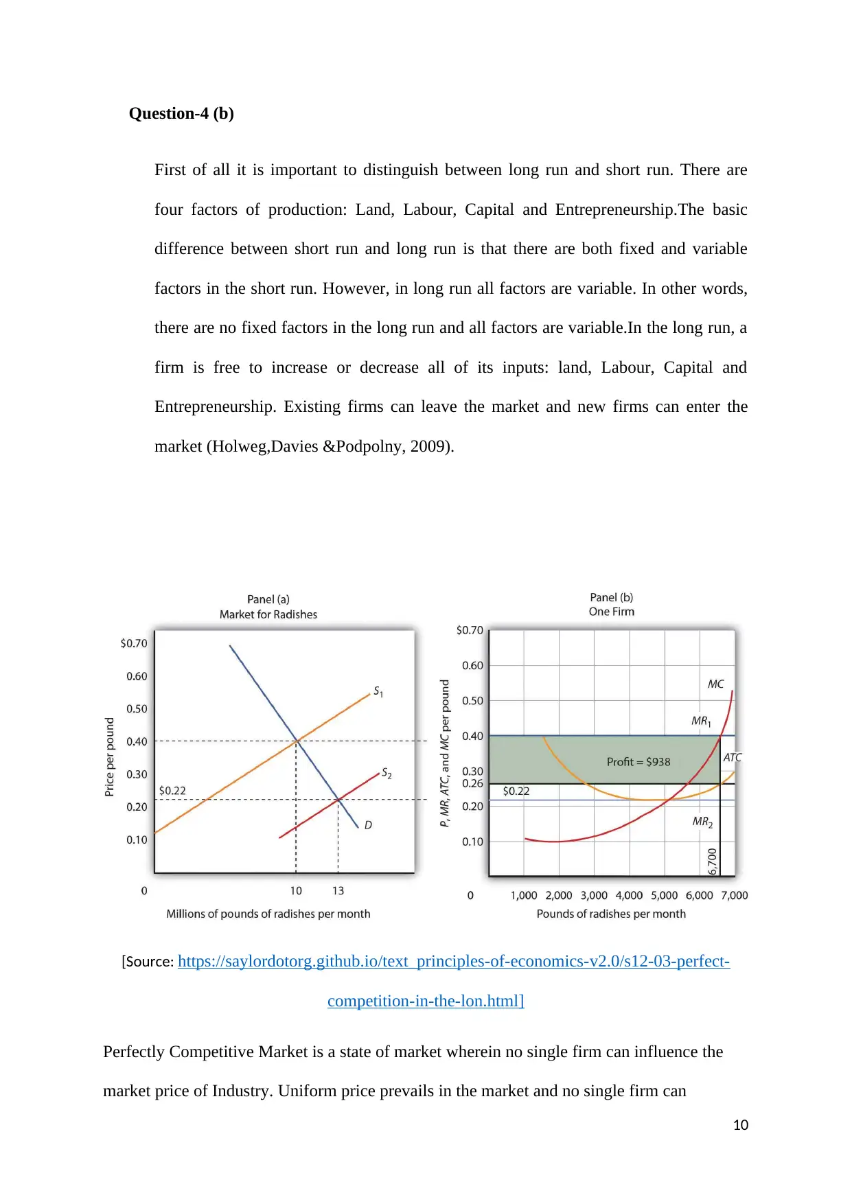
Perfectly Competitive Market is a state of market wherein no single firm can influence the
market price of Industry. Uniform price prevails in the market and no single firm can
10

influence price of Industry on its own. Adding further, Intersection of Demand and Supply
forces in the above-mentioned market decide the price of the Industry (Foster, 2014).
In the above-mentioned diagram supply curve shifted rightward. This indicates increase in
supply. As a result the equilibrium price has decreased from .40 to nearly .22
Supply refers to the quantity of a good which a producer is willing to sell at a particular price
in the market. Supply of goods at a particular price depends on the cost of factors of
Production: Land, Labour, Capital and Entrepreneurship. If price of factors of production
decreases, cost of production of goods will be fall and profit will increase. So more quantity
will be supplied at the same price. Finally, Supply curve would shift rightwards as shown in
the above diagram(Foster, 2014).
11

References:
Foster, J.B. 2014.The Theory of Monopoly Capitalism. NYU Press.
Gallardo, J.L. (2005). Comparative Advantage, Economic Growth and Free Trade MI.
Retrieved on 5th December 2017 from https://economics.ca//2009/papers/0534.pdf
Holweg, M., Davies P. &Podpolny D. (2009). The Competitive Status of the UK Automative
Industry. PICSIE Books. Retrieved on 5th December from
http://www.innovation.jbs.cam.ac.uk/research/downloads/holweg_competitive_status.pdf
Kilic, R. (2002). Absolute and Comparative Advantage: Ricardian Model. Michigan State
University, East Lansing, MI. Retrieved on 5th December 2017 from
https://msu.edu/course/ec/340/Kilic/lecture3.pdf
Langlois, R.N. (2013). Essentials of Economics. The University of Connecticut. MI.
Retrieved on 5th December 2017 fromhttp://web.uconn.edu/ciom/Supply%20and
%20Demand.pdf
Lean, M.M. & Chan P. (2011). Price Elasticity of Demand. MI. Retrieved on 5th December
2017 from http://www.yanivplan.com/files/notesonelasticity.pdf
12