ECO10250 Assignment 1: Analysis of Economic Principles, S2 2019

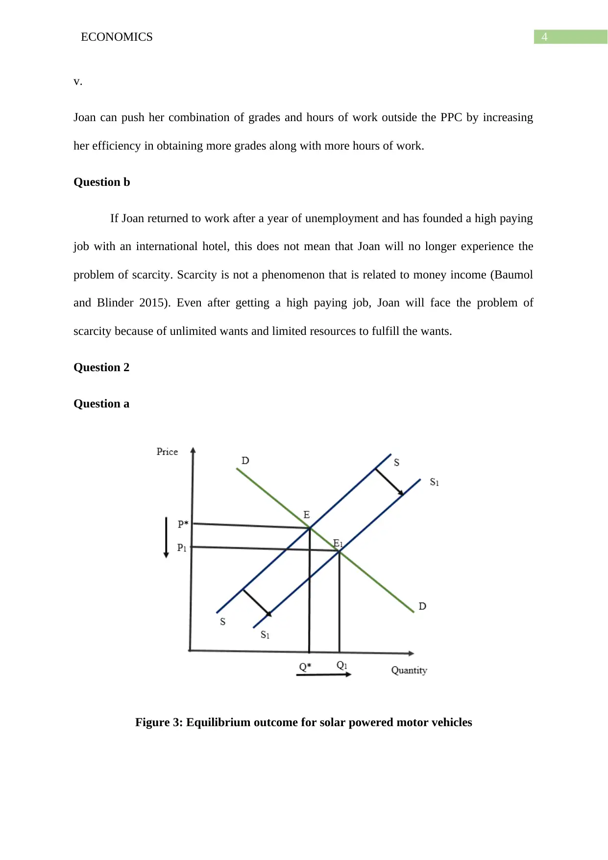
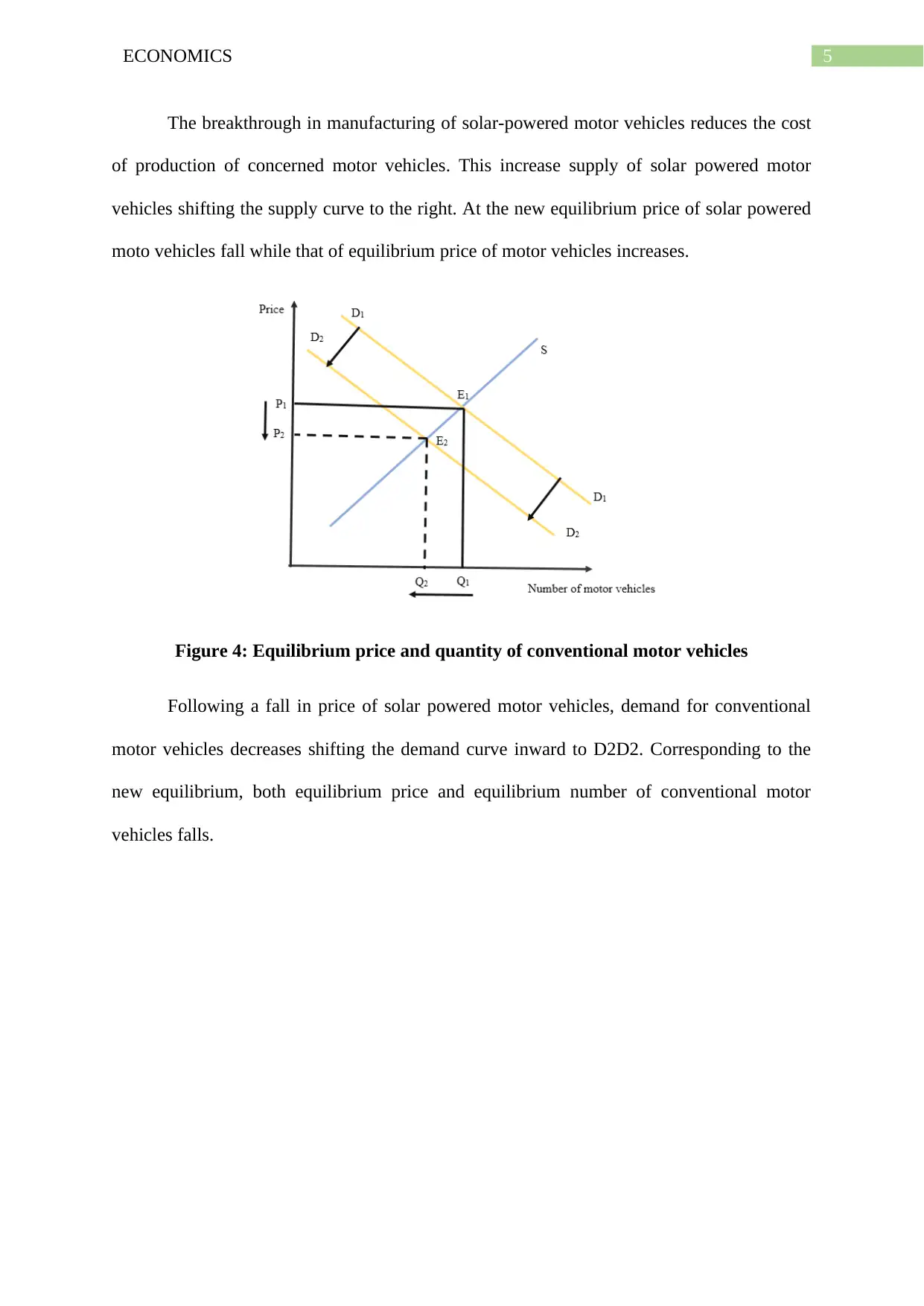
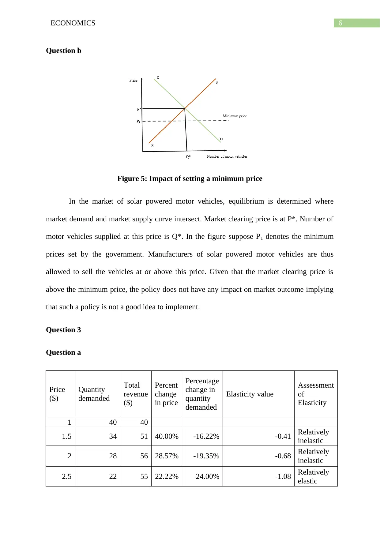
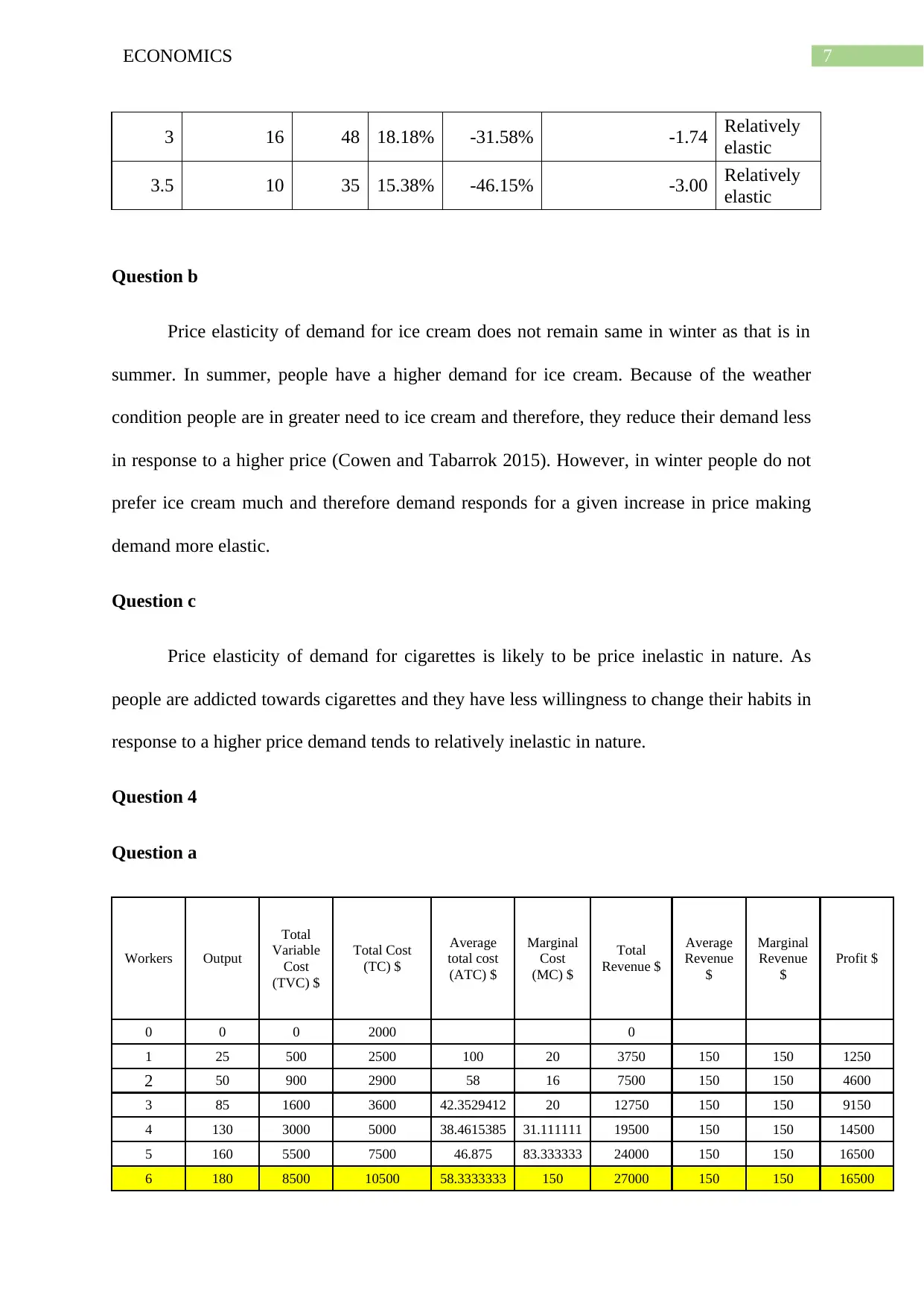
This economics assignment for ECO10250 provides detailed solutions to five questions covering core microeconomic principles. The assignment begins with an analysis of production possibility curves (PPC) and opportunity cost, illustrating how scarcity affects economic decisions. The second question examines market equilibrium, supply and demand shifts due to technological advancements and government price controls. The assignment then delves into elasticity of demand, comparing price elasticity in different scenarios, such as ice cream in summer versus winter and cigarettes. Question four explores cost structures, profit maximization, and the behavior of firms in various market conditions, including perfect competition. The final question analyzes the Australian banking sector, discussing market concentration and its implications. The assignment incorporates figures, tables, and calculations to support the economic principles discussed, providing a comprehensive understanding of microeconomics concepts.

Running head: ECONOMICS
Economics
Name of the Student
Name of the University
Course ID

1ECONOMICS
Table of Contents
Question 1..................................................................................................................................2
Question a...............................................................................................................................2
Question b..............................................................................................................................4
Question 2..................................................................................................................................4
Question a...............................................................................................................................4
Question b..............................................................................................................................6
Question 3..................................................................................................................................6
Question a...............................................................................................................................6
Question b..............................................................................................................................7
Question c...............................................................................................................................7
Question 4..................................................................................................................................7
Question a...............................................................................................................................7
Question b..............................................................................................................................8
Question c...............................................................................................................................8
Question 5..................................................................................................................................9
References................................................................................................................................11

2ECONOMICS
Question 1
Question a
i.
0 10 20 30 40 50 60 70 80 90
0
10
20
30
40
50
60
70
A
B
C
D
E
Production Possibility Curve
Grade
Work
Figure 1: Production Possibility Curve of Joan
ii.
Table 1: Increasing opportunity cost
Production Possibilities Grade Work Opportunity cost
A 0 60 0
B 20 55 0.36
C 40 45 0.89
D 60 30 2.00
E 80 0
Opportunity cost indicates unit of one good sacrifices to obtain one additional unit of another
good. At A, opportunity cost at point A is 0. At production possibilities of B, C, D and E
opportunity cost of hours of work in terms of percentage of grade increases implying an

3ECONOMICS
increasing opportunity cost along the PPC. Because of increasing opportunity cost, PPC is
concave in shape as shown in figure 1.
iii.
If the opportunity cost of Joan increasing her grade a was constant regardless of how many
hours she worked, the production possibility curve would be a straight line.
Figure 2: PPC with constant opportunity cost
The concave shape of PPC is more likely to occur because of increasing opportunity
cost. Again increasing opportunity cost occur due to scarcity of resources and also due to the
fact that resources are not equally efficient in producing all the goods (Parkin and Bade
2013). Therefore, as more and more resources shift from one good to another opportunity
cost increases.
iv.
Points inside PPC implies inefficient allocation of resources implying Joan is not efficiently
utilizing her time between grades and hours of work.

4ECONOMICS
v.
Joan can push her combination of grades and hours of work outside the PPC by increasing
her efficiency in obtaining more grades along with more hours of work.
Question b
If Joan returned to work after a year of unemployment and has founded a high paying
job with an international hotel, this does not mean that Joan will no longer experience the
problem of scarcity. Scarcity is not a phenomenon that is related to money income (Baumol
and Blinder 2015). Even after getting a high paying job, Joan will face the problem of
scarcity because of unlimited wants and limited resources to fulfill the wants.
Question 2
Question a
Figure 3: Equilibrium outcome for solar powered motor vehicles

5ECONOMICS
The breakthrough in manufacturing of solar-powered motor vehicles reduces the cost
of production of concerned motor vehicles. This increase supply of solar powered motor
vehicles shifting the supply curve to the right. At the new equilibrium price of solar powered
moto vehicles fall while that of equilibrium price of motor vehicles increases.
Figure 4: Equilibrium price and quantity of conventional motor vehicles
Following a fall in price of solar powered motor vehicles, demand for conventional
motor vehicles decreases shifting the demand curve inward to D2D2. Corresponding to the
new equilibrium, both equilibrium price and equilibrium number of conventional motor
vehicles falls.

6ECONOMICS
Question b
Figure 5: Impact of setting a minimum price
In the market of solar powered motor vehicles, equilibrium is determined where
market demand and market supply curve intersect. Market clearing price is at P*. Number of
motor vehicles supplied at this price is Q*. In the figure suppose P1 denotes the minimum
prices set by the government. Manufacturers of solar powered motor vehicles are thus
allowed to sell the vehicles at or above this price. Given that the market clearing price is
above the minimum price, the policy does not have any impact on market outcome implying
that such a policy is not a good idea to implement.
Question 3
Question a
Price
($)
Quantity
demanded
Total
revenue
($)
Percent
change
in price
Percentage
change in
quantity
demanded
Elasticity value
Assessment
of
Elasticity
1 40 40
1.5 34 51 40.00% -16.22% -0.41 Relatively
inelastic
2 28 56 28.57% -19.35% -0.68 Relatively
inelastic
2.5 22 55 22.22% -24.00% -1.08 Relatively
elastic

7ECONOMICS
3 16 48 18.18% -31.58% -1.74 Relatively
elastic
3.5 10 35 15.38% -46.15% -3.00 Relatively
elastic
Question b
Price elasticity of demand for ice cream does not remain same in winter as that is in
summer. In summer, people have a higher demand for ice cream. Because of the weather
condition people are in greater need to ice cream and therefore, they reduce their demand less
in response to a higher price (Cowen and Tabarrok 2015). However, in winter people do not
prefer ice cream much and therefore demand responds for a given increase in price making
demand more elastic.
Question c
Price elasticity of demand for cigarettes is likely to be price inelastic in nature. As
people are addicted towards cigarettes and they have less willingness to change their habits in
response to a higher price demand tends to relatively inelastic in nature.
Question 4
Question a
Workers Output
Total
Variable
Cost
(TVC) $
Total Cost
(TC) $
Average
total cost
(ATC) $
Marginal
Cost
(MC) $
Total
Revenue $
Average
Revenue
$
Marginal
Revenue
$
Profit $
0 0 0 2000 0
1 25 500 2500 100 20 3750 150 150 1250
2 50 900 2900 58 16 7500 150 150 4600
3 85 1600 3600 42.3529412 20 12750 150 150 9150
4 130 3000 5000 38.4615385 31.111111 19500 150 150 14500
5 160 5500 7500 46.875 83.333333 24000 150 150 16500
6 180 8500 10500 58.3333333 150 27000 150 150 16500

8ECONOMICS
7 195 11800 13800 70.7692308 220 29250 150 150 15450
Question b
A firm makes loss when price is less than average cost. At this price, total revenue is
less than total cost. This results in a loss to firm. However firm still continues operation as
long as price is above the minimum variable cost (Nicholson and Snyder 2014). This is
because when price is above the minimum variable cost firms are able to recover variable
cost and some of the fixed cost. However, once price falls below the minimum of average
variable cost, neither fixed cost nor the variable cost can be recovered. Firms therefore shut
down at this price.
Question c
In case of a price taking firm, firm takes market price as given. For this firm, marginal
revenue is same as average revenue. Both MR and AR equals price. Demand curve faced by
the firm is perfectly elastic. Profit maximization of the firm is subject to fulfillment of two
conditions. First is marginal cost associated with last unit produced should be equal to the
marginal cost and second marginal cost should cut the marginal revenue curve from below
(McConnell et al. 2013).

9ECONOMICS
Figure 6: Profit maximization of a price taking firm
In the above figure, profit maximization point of the firm is at E. At this point,
marginal cost is equal to price and marginal cost cuts the marginal revenue from below.
Question 5
The banking sector in Australia is highly concentrated in nature. The four biggest
banks of Australia namely ANZ Bank, Wespac, Commonwealth Bank and National Australia
Bank capturing more than 75 percent market share. Of the four banks, Westpac and
Commonwealth Bank occupies the higher share (Smyth 2019). The banking sector thus
moves closer to a monopoly market where the market is dominated by a single firm.
A market dominated by one or two firm generally harm public interest. Consumers in
the Australian banking sector are generally end up paying a high price for baking services.
Because of the limited competition consumers do not have any option to switch to other
industries (Mankiw 2014).

10ECONOMICS
Australian banking industry has more of an oligopoly market structure. Other
industries in Australia having a similar structure like Australian banking are grocery
supermarket and telecommunication industry.

11ECONOMICS
References
Baumol, W.J. and Blinder, A.S., 2015. Microeconomics: Principles and policy. Nelson
Education.
Cowell, F., 2018. Microeconomics: principles and analysis. Oxford University Press.
Cowen, T. and Tabarrok, A., 2015. Modern principles of microeconomics. Macmillan
International Higher Education.
Mankiw, N.G., 2014. Principles of economics. Cengage Learning.
McConnell, C.R., Brue, S.L., Flynn, S.M. and Grant, R.R., 2013. Microeconomics: Brief
Edition. McGraw-Hill/Irwin.
Nicholson, W. and Snyder, C.M., 2014. Intermediate microeconomics and its application.
Nelson Education.
Parkin, M. and Bade, R., 2013. Foundations of microeconomics. Pearson.
Smyth, J. 2019. Australian regulator vows to tackle ‘cosy oligopoly’ of big banks | Financial
Times. [online] Available at: https://www.ft.com/content/d940092a-25f2-11e9-8ce6-
5db4543da632 [Accessed 7 Aug. 2019].