ECO12 Macroeconomics: Job Boom, Unemployment, and Monetary Policy
VerifiedAdded on 2023/06/04
|13
|2395
|219
Report
AI Summary
This report analyzes the Australian labour market, focusing on job growth, unemployment rates, and the Reserve Bank of Australia's (RBA) monetary policy responses. It examines the relationship between job creation, labour force participation, and unemployment, highlighting the shift from full-time to part-time employment. The aggregate expenditure model is used to illustrate economic equilibrium and potential inflationary gaps. Furthermore, the report employs static and dynamic AD-AS models to assess the impact of economic growth and aggregate demand shocks on inflation and interest rates. The analysis considers the pressure on the RBA to adjust interest rates in response to job market trends and discusses the potential implications of various monetary and fiscal policies.

Running head: MACROECONOMICS
Macroeconomics
Name of the student
Name of the university
Author Note
Macroeconomics
Name of the student
Name of the university
Author Note
Paraphrase This Document
Need a fresh take? Get an instant paraphrase of this document with our AI Paraphraser
1MACROECONOMICS
Table of Contents
Answer 1 (a):...................................................................................................................................2
Answer 1 (b):...................................................................................................................................3
Answer 2:.........................................................................................................................................4
Answer 3:.........................................................................................................................................6
Answer 4:.........................................................................................................................................9
References:....................................................................................................................................11
2MACROECONOMICS
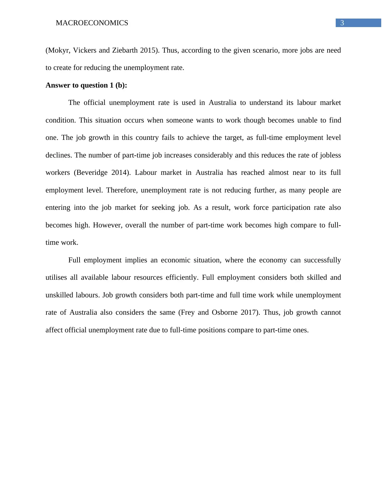
Answer to question 1 (a):
Job growth is a statistical measurement through which the government of any country can
track creation of new jobs on a monthly basis (Adelino, Ma and Robinson 2017). Hence, this
figure measures economic expansion of the country and consequently represents health of the
national economy.
Labour force participation rate, on the other side, measures the proportion of working-age
population, which actively engages within a country’s labour market. They can be engaged
through working or seeking for a job (Elsby, Hobijn and Şahin 2015). Thus, participation rate
gives the indication of available supply of labour compare to the working age population for
producing goods and services. Hence, this rate provides the distribution of the total working
force of a country.
The unemployment rate is another concept related with labour market. This rate
represents the share of total labour force, which is jobless, in terms of percentage. This rate is
considered as a lagging indicator, which implies measurable economic factor. This factor
changes when the economy starts to follow a specific trend (Theut Riis, Thorlacius, Knudsen
List and Jemec 2017). Thus, this unemployment rate rise when the economy experiences poor
conditions and jobs become scarce. On the contrary, if the economy follows a healthy rate as
well as huge number of jobs, then this rate could be decreased. In this context, it can be
mentioned that labour force participation rate and unemployment rate has opposite relation.
Thus, these three indicators has close link through which labour market of Australia can
be described. Through job growth, the economy can increase its labour force participation rate in
job market. This in turn can reduce the unemployment rate and represent a healthy labour market
⊘ This is a preview!⊘
Do you want full access?
Subscribe today to unlock all pages.
Trusted by 1+ million students worldwide
3MACROECONOMICS
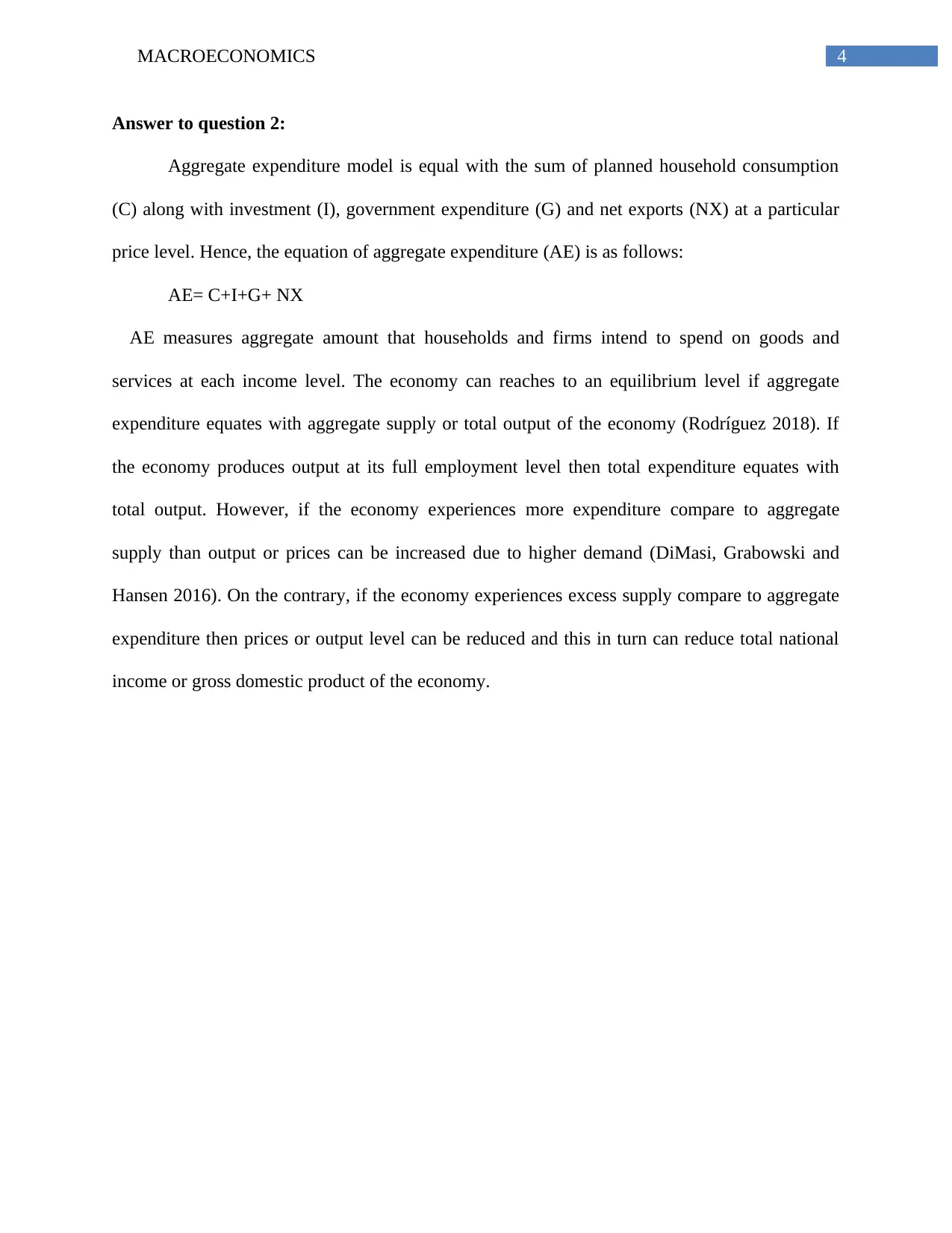
(Mokyr, Vickers and Ziebarth 2015). Thus, according to the given scenario, more jobs are need
to create for reducing the unemployment rate.
Answer to question 1 (b):
The official unemployment rate is used in Australia to understand its labour market
condition. This situation occurs when someone wants to work though becomes unable to find
one. The job growth in this country fails to achieve the target, as full-time employment level
declines. The number of part-time job increases considerably and this reduces the rate of jobless
workers (Beveridge 2014). Labour market in Australia has reached almost near to its full
employment level. Therefore, unemployment rate is not reducing further, as many people are
entering into the job market for seeking job. As a result, work force participation rate also
becomes high. However, overall the number of part-time work becomes high compare to full-
time work.
Full employment implies an economic situation, where the economy can successfully
utilises all available labour resources efficiently. Full employment considers both skilled and
unskilled labours. Job growth considers both part-time and full time work while unemployment
rate of Australia also considers the same (Frey and Osborne 2017). Thus, job growth cannot
affect official unemployment rate due to full-time positions compare to part-time ones.
Paraphrase This Document
Need a fresh take? Get an instant paraphrase of this document with our AI Paraphraser
4MACROECONOMICS
Answer to question 2:
Aggregate expenditure model is equal with the sum of planned household consumption
(C) along with investment (I), government expenditure (G) and net exports (NX) at a particular
price level. Hence, the equation of aggregate expenditure (AE) is as follows:
AE= C+I+G+ NX
AE measures aggregate amount that households and firms intend to spend on goods and
services at each income level. The economy can reaches to an equilibrium level if aggregate
expenditure equates with aggregate supply or total output of the economy (Rodríguez 2018). If
the economy produces output at its full employment level then total expenditure equates with
total output. However, if the economy experiences more expenditure compare to aggregate
supply than output or prices can be increased due to higher demand (DiMasi, Grabowski and
Hansen 2016). On the contrary, if the economy experiences excess supply compare to aggregate
expenditure then prices or output level can be reduced and this in turn can reduce total national
income or gross domestic product of the economy.
5MACROECONOMICS
Aggregate expenditure
Total Output
AE
Qf
AEf
Aggregate supply
Qp
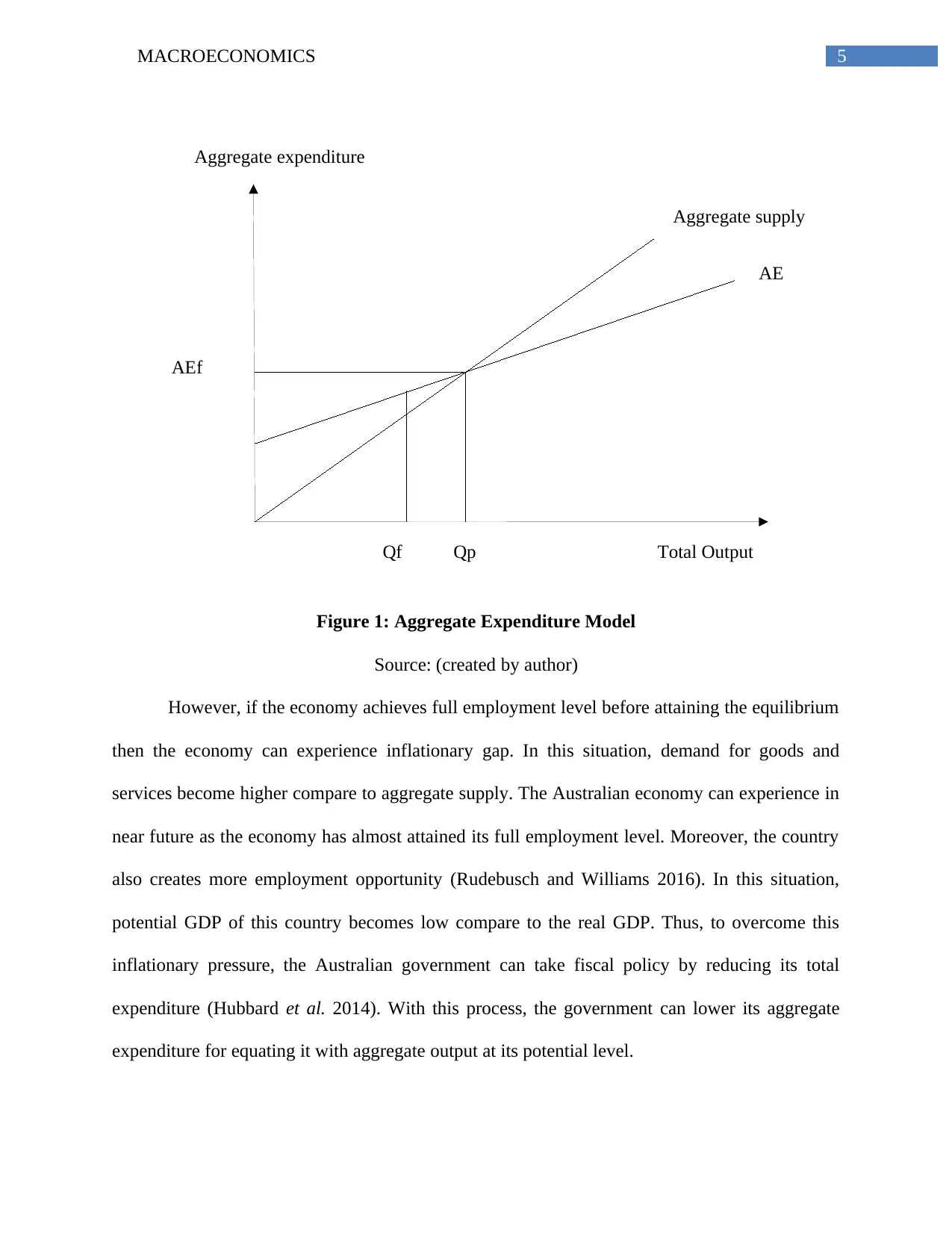
Figure 1: Aggregate Expenditure Model
Source: (created by author)
However, if the economy achieves full employment level before attaining the equilibrium
then the economy can experience inflationary gap. In this situation, demand for goods and
services become higher compare to aggregate supply. The Australian economy can experience in
near future as the economy has almost attained its full employment level. Moreover, the country
also creates more employment opportunity (Rudebusch and Williams 2016). In this situation,
potential GDP of this country becomes low compare to the real GDP. Thus, to overcome this
inflationary pressure, the Australian government can take fiscal policy by reducing its total
expenditure (Hubbard et al. 2014). With this process, the government can lower its aggregate
expenditure for equating it with aggregate output at its potential level.
Aggregate expenditure
Total Output
AE
Qf
AEf
Aggregate supply
Qp
Figure 1: Aggregate Expenditure Model
Source: (created by author)
However, if the economy achieves full employment level before attaining the equilibrium
then the economy can experience inflationary gap. In this situation, demand for goods and
services become higher compare to aggregate supply. The Australian economy can experience in
near future as the economy has almost attained its full employment level. Moreover, the country
also creates more employment opportunity (Rudebusch and Williams 2016). In this situation,
potential GDP of this country becomes low compare to the real GDP. Thus, to overcome this
inflationary pressure, the Australian government can take fiscal policy by reducing its total
expenditure (Hubbard et al. 2014). With this process, the government can lower its aggregate
expenditure for equating it with aggregate output at its potential level.
⊘ This is a preview!⊘
Do you want full access?
Subscribe today to unlock all pages.
Trusted by 1+ million students worldwide
6MACROECONOMICS
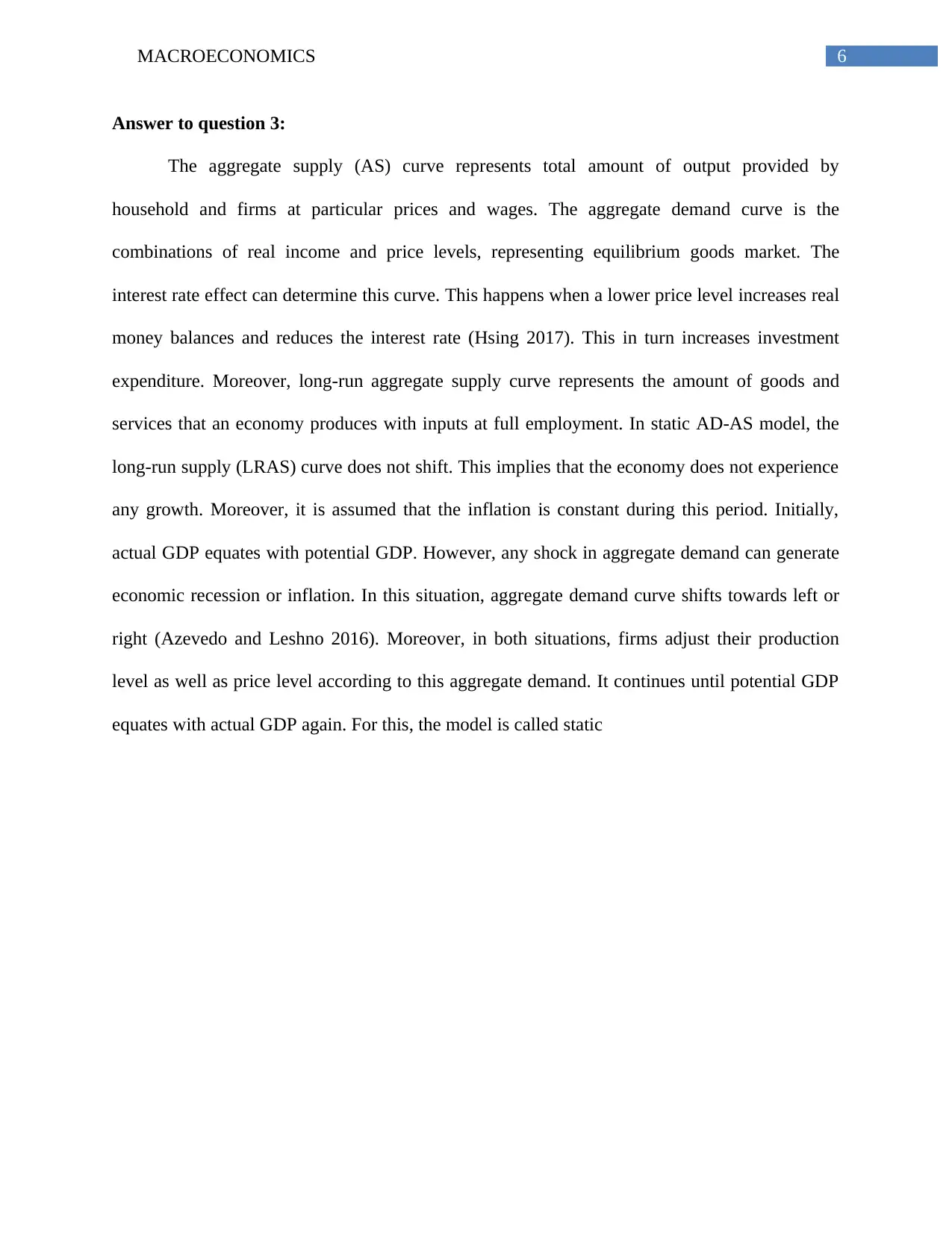
Answer to question 3:
The aggregate supply (AS) curve represents total amount of output provided by
household and firms at particular prices and wages. The aggregate demand curve is the
combinations of real income and price levels, representing equilibrium goods market. The
interest rate effect can determine this curve. This happens when a lower price level increases real
money balances and reduces the interest rate (Hsing 2017). This in turn increases investment
expenditure. Moreover, long-run aggregate supply curve represents the amount of goods and
services that an economy produces with inputs at full employment. In static AD-AS model, the
long-run supply (LRAS) curve does not shift. This implies that the economy does not experience
any growth. Moreover, it is assumed that the inflation is constant during this period. Initially,
actual GDP equates with potential GDP. However, any shock in aggregate demand can generate
economic recession or inflation. In this situation, aggregate demand curve shifts towards left or
right (Azevedo and Leshno 2016). Moreover, in both situations, firms adjust their production
level as well as price level according to this aggregate demand. It continues until potential GDP
equates with actual GDP again. For this, the model is called static
Paraphrase This Document
Need a fresh take? Get an instant paraphrase of this document with our AI Paraphraser
7MACROECONOMICS
Real GDP
Price level LAS
P0
O
SRAS0
AD0
Qp
AD1
SRAS1
P1
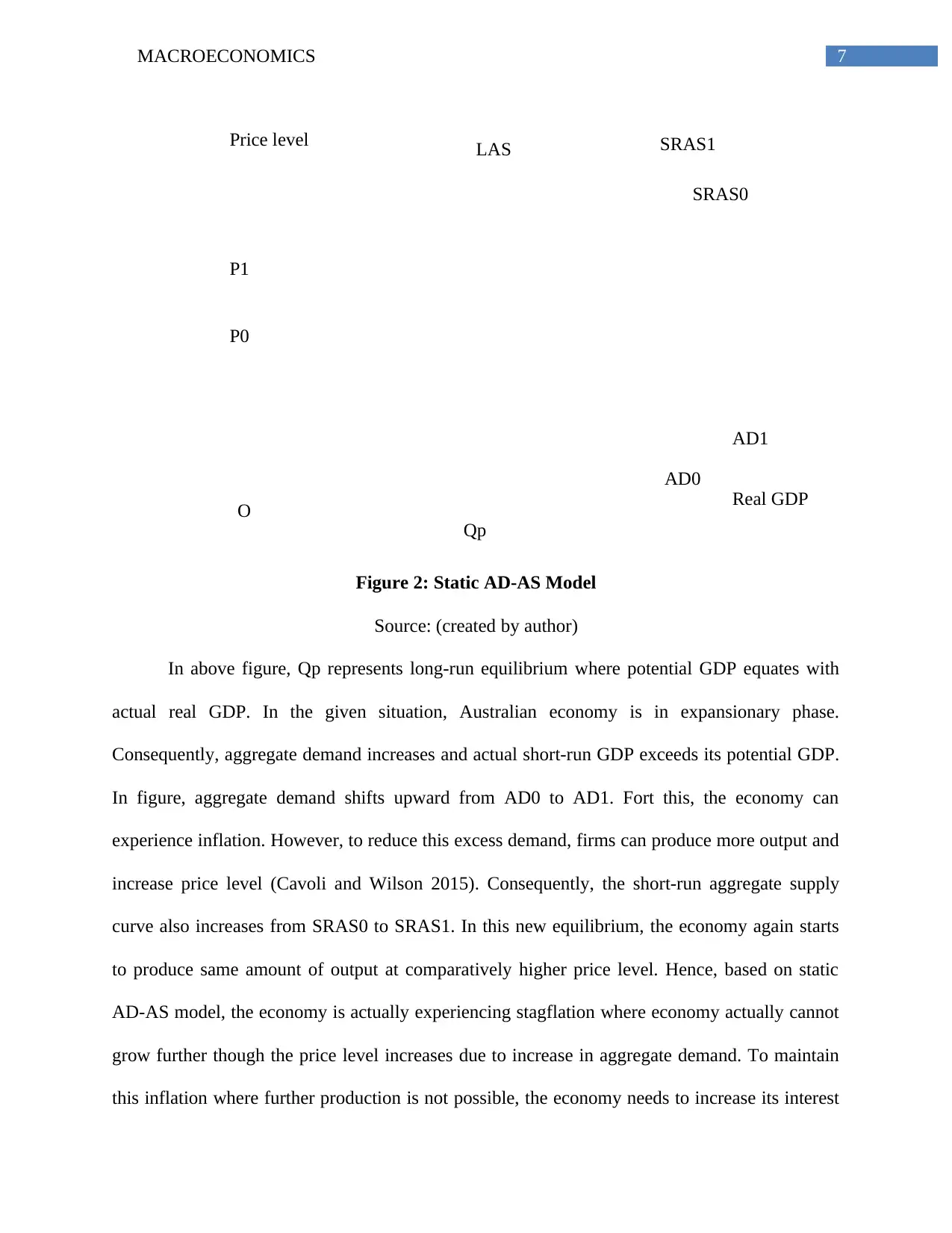
Figure 2: Static AD-AS Model
Source: (created by author)
In above figure, Qp represents long-run equilibrium where potential GDP equates with
actual real GDP. In the given situation, Australian economy is in expansionary phase.
Consequently, aggregate demand increases and actual short-run GDP exceeds its potential GDP.
In figure, aggregate demand shifts upward from AD0 to AD1. Fort this, the economy can
experience inflation. However, to reduce this excess demand, firms can produce more output and
increase price level (Cavoli and Wilson 2015). Consequently, the short-run aggregate supply
curve also increases from SRAS0 to SRAS1. In this new equilibrium, the economy again starts
to produce same amount of output at comparatively higher price level. Hence, based on static
AD-AS model, the economy is actually experiencing stagflation where economy actually cannot
grow further though the price level increases due to increase in aggregate demand. To maintain
this inflation where further production is not possible, the economy needs to increase its interest
Real GDP
Price level LAS
P0
O
SRAS0
AD0
Qp
AD1
SRAS1
P1
Figure 2: Static AD-AS Model
Source: (created by author)
In above figure, Qp represents long-run equilibrium where potential GDP equates with
actual real GDP. In the given situation, Australian economy is in expansionary phase.
Consequently, aggregate demand increases and actual short-run GDP exceeds its potential GDP.
In figure, aggregate demand shifts upward from AD0 to AD1. Fort this, the economy can
experience inflation. However, to reduce this excess demand, firms can produce more output and
increase price level (Cavoli and Wilson 2015). Consequently, the short-run aggregate supply
curve also increases from SRAS0 to SRAS1. In this new equilibrium, the economy again starts
to produce same amount of output at comparatively higher price level. Hence, based on static
AD-AS model, the economy is actually experiencing stagflation where economy actually cannot
grow further though the price level increases due to increase in aggregate demand. To maintain
this inflation where further production is not possible, the economy needs to increase its interest

8MACROECONOMICS
rate. If the Reserve bank of Australia (RBA) cannot increase this interest rate then the price level
even increases further with no economic growth (Leduc and Liu 2016). Thus, according to
analysts, job boom in Australian market may pressurise the RBA to increase its interest rate.
However, economists suggest that RBA is not increasing its cash rate up to 2020.
⊘ This is a preview!⊘
Do you want full access?
Subscribe today to unlock all pages.
Trusted by 1+ million students worldwide
9MACROECONOMICS
Price level
O Real output
Q0 Q1+
SRAS0
SRAS1
AD0
LRAS0 LRAS1
AD1
AD3
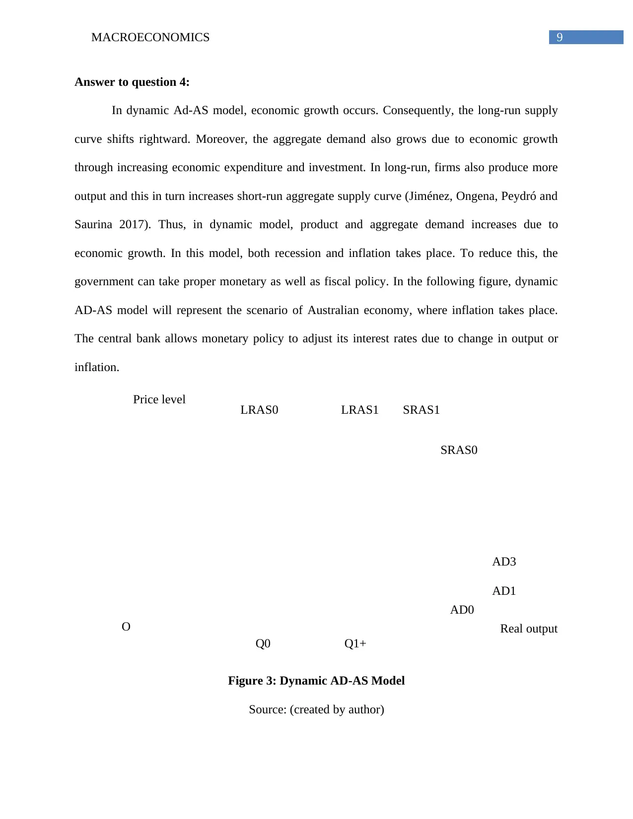
Answer to question 4:
In dynamic Ad-AS model, economic growth occurs. Consequently, the long-run supply
curve shifts rightward. Moreover, the aggregate demand also grows due to economic growth
through increasing economic expenditure and investment. In long-run, firms also produce more
output and this in turn increases short-run aggregate supply curve (Jiménez, Ongena, Peydró and
Saurina 2017). Thus, in dynamic model, product and aggregate demand increases due to
economic growth. In this model, both recession and inflation takes place. To reduce this, the
government can take proper monetary as well as fiscal policy. In the following figure, dynamic
AD-AS model will represent the scenario of Australian economy, where inflation takes place.
The central bank allows monetary policy to adjust its interest rates due to change in output or
inflation.
Figure 3: Dynamic AD-AS Model
Source: (created by author)
Price level
O Real output
Q0 Q1+
SRAS0
SRAS1
AD0
LRAS0 LRAS1
AD1
AD3
Answer to question 4:
In dynamic Ad-AS model, economic growth occurs. Consequently, the long-run supply
curve shifts rightward. Moreover, the aggregate demand also grows due to economic growth
through increasing economic expenditure and investment. In long-run, firms also produce more
output and this in turn increases short-run aggregate supply curve (Jiménez, Ongena, Peydró and
Saurina 2017). Thus, in dynamic model, product and aggregate demand increases due to
economic growth. In this model, both recession and inflation takes place. To reduce this, the
government can take proper monetary as well as fiscal policy. In the following figure, dynamic
AD-AS model will represent the scenario of Australian economy, where inflation takes place.
The central bank allows monetary policy to adjust its interest rates due to change in output or
inflation.
Figure 3: Dynamic AD-AS Model
Source: (created by author)
Paraphrase This Document
Need a fresh take? Get an instant paraphrase of this document with our AI Paraphraser
10MACROECONOMICS
The dynamic aggregate supply curve will shift to the right, as the Australian economy is
going to produce more goods and services. In addition to this, aggregate demand curve also
increases. Thus, the economy is producing its output and consequently aggregate demand curve
shifts from AD0 to AD1. However, due to increase in long-run aggregate supply curve, the
economy may perform at recession (Michaillat and Saez 2015). Hence, to obtain equilibrium
again, the Australian government needs to increase its aggregate demand up to AD3. To do so,
the government can take effective monetary or fiscal policy (Hubbard et al. 2014). However, the
aggregate price level will also increase and this further can cause inflation. Thus, to reduce this
situation, the RBA may increase its cash rate.
11MACROECONOMICS
References:
Adelino, M., Ma, S. and Robinson, D., 2017. Firm age, investment opportunities, and job
creation. The Journal of Finance, 72(3), pp.999-1038.
Azevedo, E.M. and Leshno, J.D., 2016. A supply and demand framework for two-sided
matching markets. Journal of Political Economy, 124(5), pp.1235-1268.
Beveridge, W.H., 2014. Full Employment in a Free Society (Works of William H. Beveridge): A
Report. Routledge.
Cavoli, T. and Wilson, J.K., 2015. Corruption, central bank (in) dependence and optimal
monetary policy in a simple model. Journal of Policy Modeling, 37(3), pp.501-509.
DiMasi, J.A., Grabowski, H.G. and Hansen, R.W., 2016. Innovation in the pharmaceutical
industry: new estimates of R&D costs. Journal of health economics, 47, pp.20-33.
Elsby, M.W., Hobijn, B. and Şahin, A., 2015. On the importance of the participation margin for
labor market fluctuations. Journal of Monetary Economics, 72, pp.64-82.
Frey, C.B. and Osborne, M.A., 2017. The future of employment: how susceptible are jobs to
computerisation?. Technological forecasting and social change, 114, pp.254-280.
Hsing, Y., 2017. Is Currency Depreciation or More Government Debt Expansionary? The Case
of Thailand. Journal of Advances in Economics and Finance, 2(4), p.237.
Hubbard, G., Garnett, A., Lewis, P. and O’Brien, A., 2014. Essentials of Economics. Pearson
Australia Pty Ltd
Jiménez, G., Ongena, S., Peydró, J.L. and Saurina, J., 2017. Macroprudential policy,
countercyclical bank capital buffers, and credit supply: evidence from the Spanish dynamic
provisioning experiments. Journal of Political Economy, 125(6), pp.2126-2177.
⊘ This is a preview!⊘
Do you want full access?
Subscribe today to unlock all pages.
Trusted by 1+ million students worldwide
1 out of 13
Related Documents


Your All-in-One AI-Powered Toolkit for Academic Success.
+13062052269
info@desklib.com
Available 24*7 on WhatsApp / Email
![[object Object]](/_next/static/media/star-bottom.7253800d.svg)
Unlock your academic potential
Copyright © 2020–2026 A2Z Services. All Rights Reserved. Developed and managed by ZUCOL.