La Trobe University: Economic Growth and Stability - ECO3EGS Report
VerifiedAdded on 2023/06/16
|11
|2417
|381
Report
AI Summary
This report provides an analysis of economic growth and stability, focusing on the Solow Growth Model. It includes analytical work, computational simulations using MS-Excel to assess policy changes, and an interpretation of the empirical research paper 'A Contribution to the Empirics of Economic Growth' by Mankiw, Romer, and Weil. The report delves into steady-state and Golden-Rule steady-state levels, examines the impact of unemployment, and explores the role of human capital in economic growth. Key transformations, estimations, and potential improvements to the model are discussed, providing a comprehensive understanding of the factors influencing economic growth and stability.
qwertyuiopasdfghjklzxcvbnmq
wertyuiopasdfghjklzxcvbnmqw
ertyuiopasdfghjklzxcvbnmqwe
rtyuiopasdfghjklzxcvbnmqwert
yuiopasdfghjklzxcvbnmqwerty
uiopasdfghjklzxcvbnmqwertyui
opasdfghjklzxcvbnmqwertyuio
pasdfghjklzxcvbnmqwertyuiop
asdfghjklzxcvbnmqwertyuiopa
sdfghjklzxcvbnmqwertyuiopas
dfghjklzxcvbnmqwertyuiopasd
fghjklzxcvbnmqwertyuiopasdf
ghjklzxcvbnmqwertyuiopasdfg
hjklzxcvbnmqwertyuiopasdfghj
klzxcvbnmqwertyuiopasdfghjkl
zxcvbnmqwertyuiopasdfghjklz
xcvbnmqwertyuiopasdfghjklzx
cvbnmrtyuiopasdfghjklzxcvbn
mqwertyuiopasdfghjklzxcvbn
(
Economic Growth and Stability: Theory and Evidence
[Type the document subtitle]
12/10/2017
ABC
Paraphrase This Document
Need a fresh take? Get an instant paraphrase of this document with our AI Paraphraser

Contents
1
Part A: Analytical Work.................................................................................................................................. 3
ssGolden-Rule Steady State........................................................................................................................... 4
Unemployment in the Solow Model............................................................................................................ 5
Part B: Computational Work.......................................................................................................................... 5
Part C: A Contribution to the Empirics of Economic Growth. Solow Model with
Human Capital.................................................................................................................................................... 7
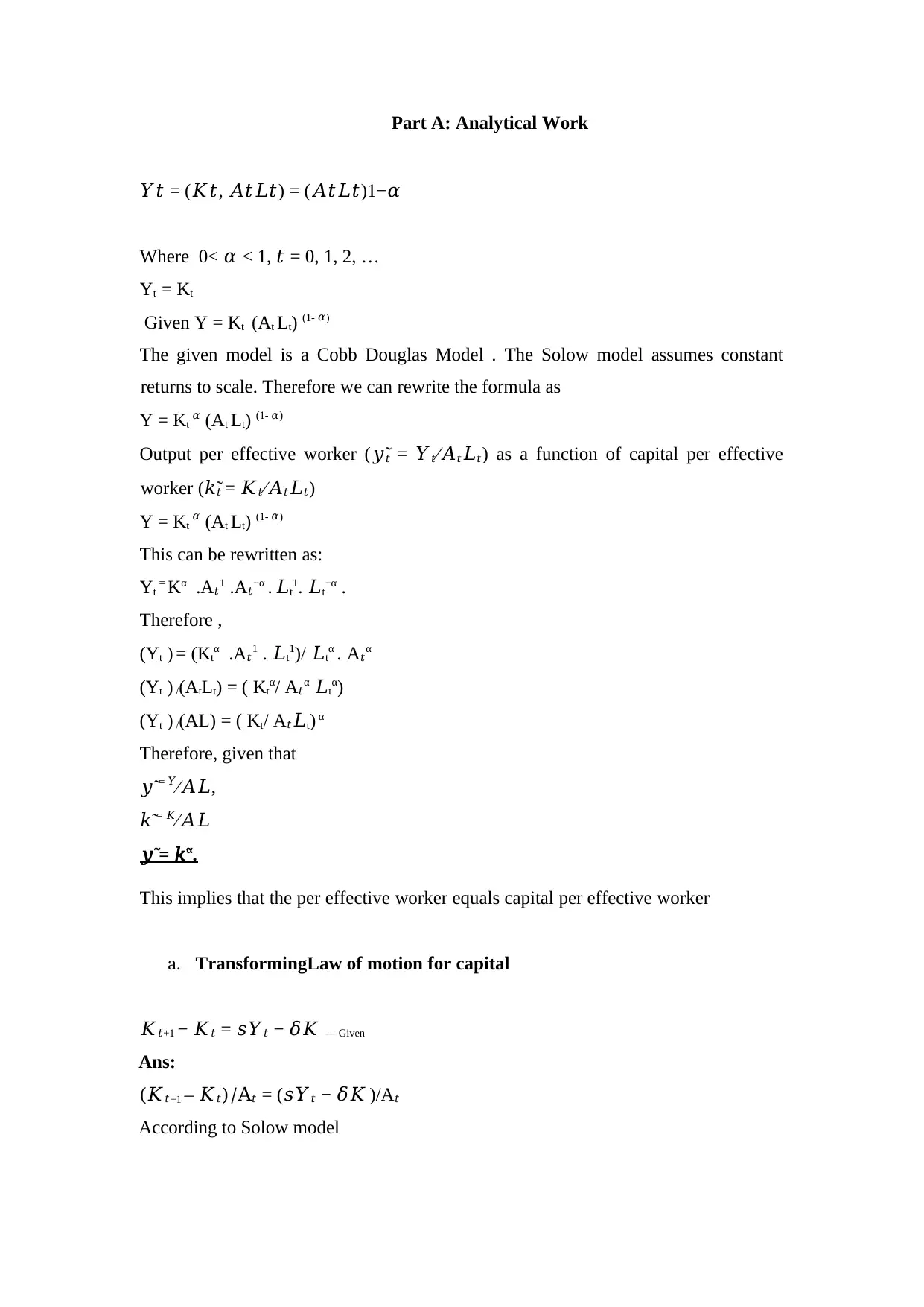
Part A: Analytical Work
𝑌𝑡 = (𝐾𝑡, 𝐴𝑡𝐿𝑡) = (𝐴𝑡𝐿𝑡)1−𝛼
Where 0< 𝛼 < 1, 𝑡 = 0, 1, 2, …
Yt = Kt
Given Y = Kt (At Lt) (1- 𝛼)
The given model is a Cobb Douglas Model . The Solow model assumes constant
returns to scale. Therefore we can rewrite the formula as
Y = Kt 𝛼 (At Lt) (1- 𝛼)
Output per effective worker (𝑦̃ 𝑡 = 𝑌𝑡⁄𝐴𝑡𝐿𝑡) as a function of capital per effective
worker (𝑘̃𝑡 = 𝐾𝑡⁄𝐴𝑡𝐿𝑡)
Y = Kt 𝛼 (At Lt) (1- 𝛼)
This can be rewritten as:
Yt = Kα .A𝑡1 .A𝑡−α . 𝐿t1. 𝐿t−α .
Therefore ,
(Yt ) = (Ktα .A𝑡1 . 𝐿t1)/ 𝐿tα . A𝑡α
(Yt ) /(AtLt) = ( Ktα/ A𝑡α 𝐿tα)
(Yt ) /(AL) = ( Kt/ A𝑡𝐿t) α
Therefore, given that
𝑦̃ = 𝑌⁄𝐴𝐿,
𝑘̃ = 𝐾⁄𝐴𝐿
𝑦̃ = 𝑘̃α.
This implies that the per effective worker equals capital per effective worker
a. TransformingLaw of motion for capital
𝐾𝑡+1 − 𝐾𝑡 = 𝑠𝑌𝑡 − 𝛿𝐾 --- Given
Ans:
(𝐾𝑡+1 – 𝐾𝑡)/A𝑡 = (𝑠𝑌𝑡 − 𝛿𝐾 )/A𝑡
According to Solow model
⊘ This is a preview!⊘
Do you want full access?
Subscribe today to unlock all pages.
Trusted by 1+ million students worldwide
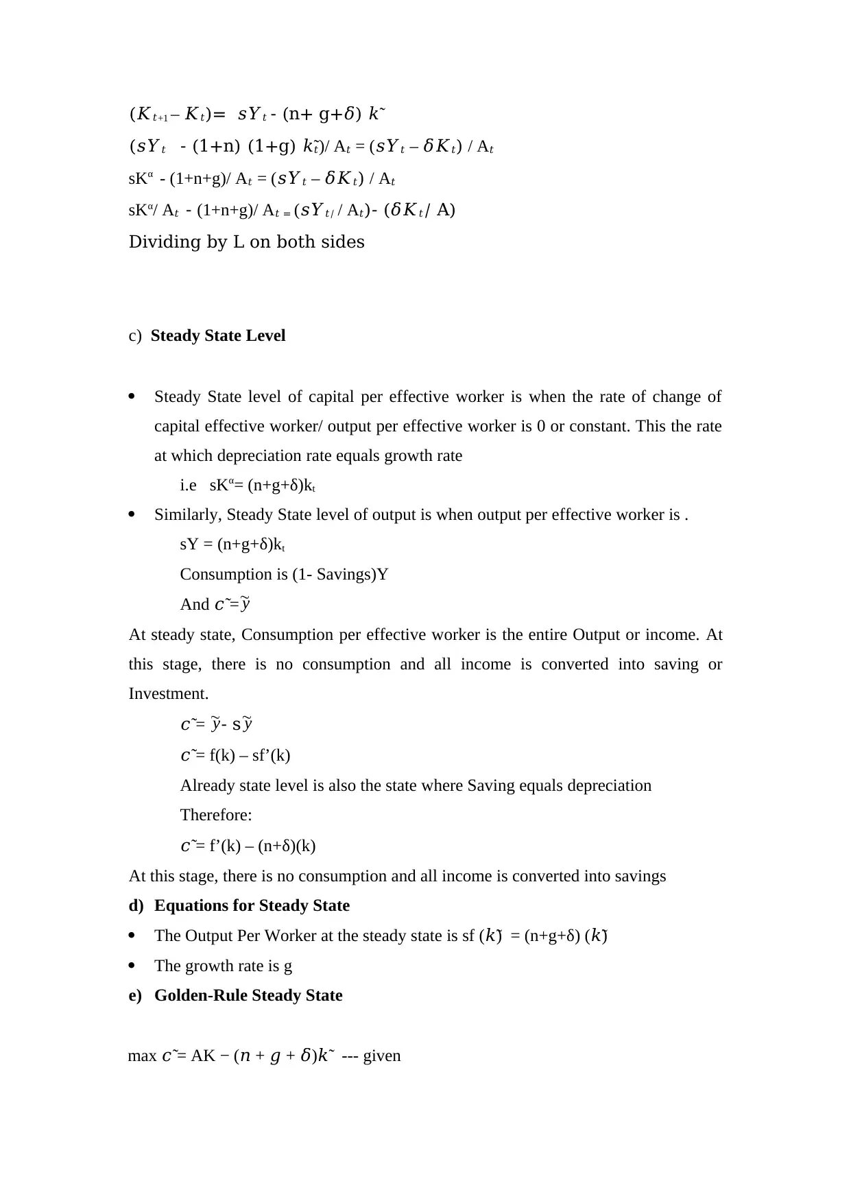
(𝐾𝑡+1 – 𝐾𝑡)= 𝑠𝑌𝑡 - (n+ g+𝛿) 𝑘̃
(𝑠𝑌𝑡 - (1+n) (1+g) 𝑘̃𝑡)/ A𝑡 = (𝑠𝑌𝑡 – 𝛿𝐾𝑡) / A𝑡
sKα - (1+n+g)/ A𝑡 = (𝑠𝑌𝑡 – 𝛿𝐾𝑡) / A𝑡
sKα/ A𝑡 - (1+n+g)/ A𝑡 = (𝑠𝑌𝑡/ / A𝑡)- (𝛿𝐾𝑡/ A)
Dividing by L on both sides
c) Steady State Level
Steady State level of capital per effective worker is when the rate of change of
capital effective worker/ output per effective worker is 0 or constant. This the rate
at which depreciation rate equals growth rate
i.e sKα= (n+g+δ)kt
Similarly, Steady State level of output is when output per effective worker is .
sY = (n+g+δ)kt
Consumption is (1- Savings)Y
And 𝑐̃ =~y
At steady state, Consumption per effective worker is the entire Output or income. At
this stage, there is no consumption and all income is converted into saving or
Investment.
𝑐̃ = ~y- s~y
𝑐̃ = f(k) – sf’(k)
Already state level is also the state where Saving equals depreciation
Therefore:
𝑐̃ = f’(k) – (n+δ)(k)
At this stage, there is no consumption and all income is converted into savings
d) Equations for Steady State
The Output Per Worker at the steady state is sf (𝑘̃) = (n+g+δ) (𝑘̃)
The growth rate is g
e) Golden-Rule Steady State
max 𝑐̃ = AK − (𝑛 + 𝑔 + 𝛿)𝑘̃ --- given
Paraphrase This Document
Need a fresh take? Get an instant paraphrase of this document with our AI Paraphraser
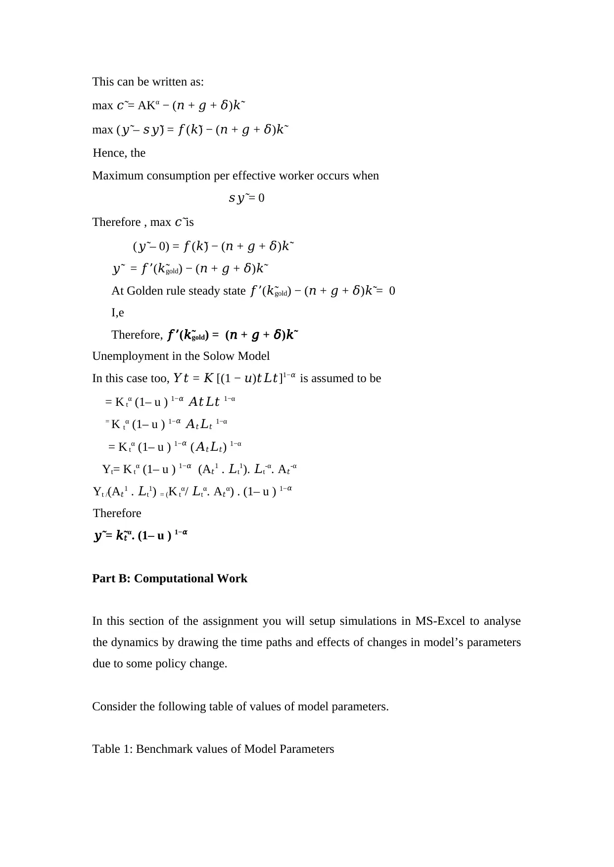
This can be written as:
max 𝑐̃ = AKα − (𝑛 + 𝑔 + 𝛿)𝑘̃
max (𝑦̃ – 𝑠𝑦̃ ) = 𝑓(𝑘̃) − (𝑛 + 𝑔 + 𝛿)𝑘̃
Hence, the
Maximum consumption per effective worker occurs when
𝑠𝑦̃ = 0
Therefore , max 𝑐̃ is
(𝑦̃ – 0) = 𝑓(𝑘̃) − (𝑛 + 𝑔 + 𝛿)𝑘̃
𝑦̃ = 𝑓’(𝑘̃gold) − (𝑛 + 𝑔 + 𝛿)𝑘̃
At Golden rule steady state 𝑓’(𝑘̃gold) − (𝑛 + 𝑔 + 𝛿)𝑘̃ = 0
I,e
Therefore, 𝑓’(𝑘̃gold) = (𝑛 + 𝑔 + 𝛿)𝑘̃
Unemployment in the Solow Model
In this case too, 𝑌𝑡 = 𝐾 [(1 − 𝑢)𝑡𝐿𝑡]1−𝛼 is assumed to be
= K tα (1– u ) 1−𝛼 𝐴𝑡𝐿𝑡 1−α
= K tα (1– u ) 1−𝛼 𝐴𝑡𝐿𝑡 1−α
= K tα (1– u ) 1−𝛼 (𝐴𝑡𝐿𝑡) 1−α
Yt= K tα (1– u ) 1−𝛼 (A𝑡1 . 𝐿t1). 𝐿t-α. A𝑡-α
Yt /(A𝑡1 . 𝐿t1) = (K tα/ 𝐿tα. A𝑡α) . (1– u ) 1−𝛼
Therefore
𝑦̃ = 𝑘̃𝑡α. (1– u ) 1−𝛼
Part B: Computational Work
In this section of the assignment you will setup simulations in MS-Excel to analyse
the dynamics by drawing the time paths and effects of changes in model’s parameters
due to some policy change.
Consider the following table of values of model parameters.
Table 1: Benchmark values of Model Parameters

g. Use above parameters values to obtain the steady state levels of
𝑘̃, 𝑦̃, 𝑐̃, 𝑘̃𝑔𝑜𝑙𝑑, 𝑦̃𝑔𝑜𝑙𝑑and 𝑐𝑔𝑜𝑙𝑑̃ (You can do this on paper using calculator).
.
𝑘̃ = 1.4196669143975
𝑦̃ = 1.123902974
𝑐̃𝑡 = 0.98903461712
𝑘̃𝑔𝑜𝑙𝑑 =0.134868356867764
𝑦̃ 𝑔𝑜𝑙𝑑= 0.512825984
𝑐𝑔𝑜𝑙𝑑̃ = 0.451286866053635
Capital, output and consumption keep growing with diminishing returns qhich
is reflected in an upward rising curve that becomes flat as it grows. They take
a slight dip, when savings rate are increased. However, due to the
accumulation of capital, the curve rises again. The initial value of technology
curve is flat since it is a constant. curve is flat.
However, capital stock rises due to an increase in savings rate since savings
are converted into capital stock.
Calculations in excel sheet
h)
Capital per worker because capital because rates are too high for
investment. However, in our model ,we have assumed savings=
investment. So capital per workers increases.
Output per workers also increases. Out out increases because 𝑘̃ has
increased while L remains same.
Consumption per worker declines briefly but then begins to increase.
This is due to the fact that savings are converted into investments.
⊘ This is a preview!⊘
Do you want full access?
Subscribe today to unlock all pages.
Trusted by 1+ million students worldwide
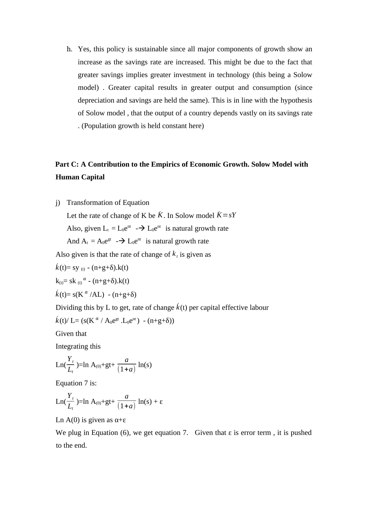
h. Yes, this policy is sustainable since all major components of growth show an
increase as the savings rate are increased. This might be due to the fact that
greater savings implies greater investment in technology (this being a Solow
model) . Greater capital results in greater output and consumption (since
depreciation and savings are held the same). This is in line with the hypothesis
of Solow model , that the output of a country depends vastly on its savings rate
. (Population growth is held constant here)
Part C: A Contribution to the Empirics of Economic Growth. Solow Model with
Human Capital
j) Transformation of Equation
Let the rate of change of K be ˙K . In Solow model ˙K=sY
Also, given Lt = L0ent - L0ent is natural growth rate
And At = A0egt - L0ent is natural growth rate
Also given is that the rate of change of k t is given as
˙k(t)= sy (t) - (n+g+δ).k(t)
k(t)= sk (t) 𝛼 - (n+g+δ).k(t)
˙k(t)= s(K 𝛼 /AL) - (n+g+δ)
Dividing this by L to get, rate of change ˙k(t) per capital effective labour
˙k(t)/ L= (s(K 𝛼 / A0egt .L0ent ) - (n+g+δ))
Given that
Integrating this
Ln( Y t
Lt
)=ln A(0)+gt+ a
(1+a) ln(s)
Equation 7 is:
Ln( Y t
Lt
)=ln A(0)+gt+ a
(1+a) ln(s) + ε
Ln A(0) is given as α+ε
We plug in Equation (6), we get equation 7. Given that ε is error term , it is pushed
to the end.
Paraphrase This Document
Need a fresh take? Get an instant paraphrase of this document with our AI Paraphraser
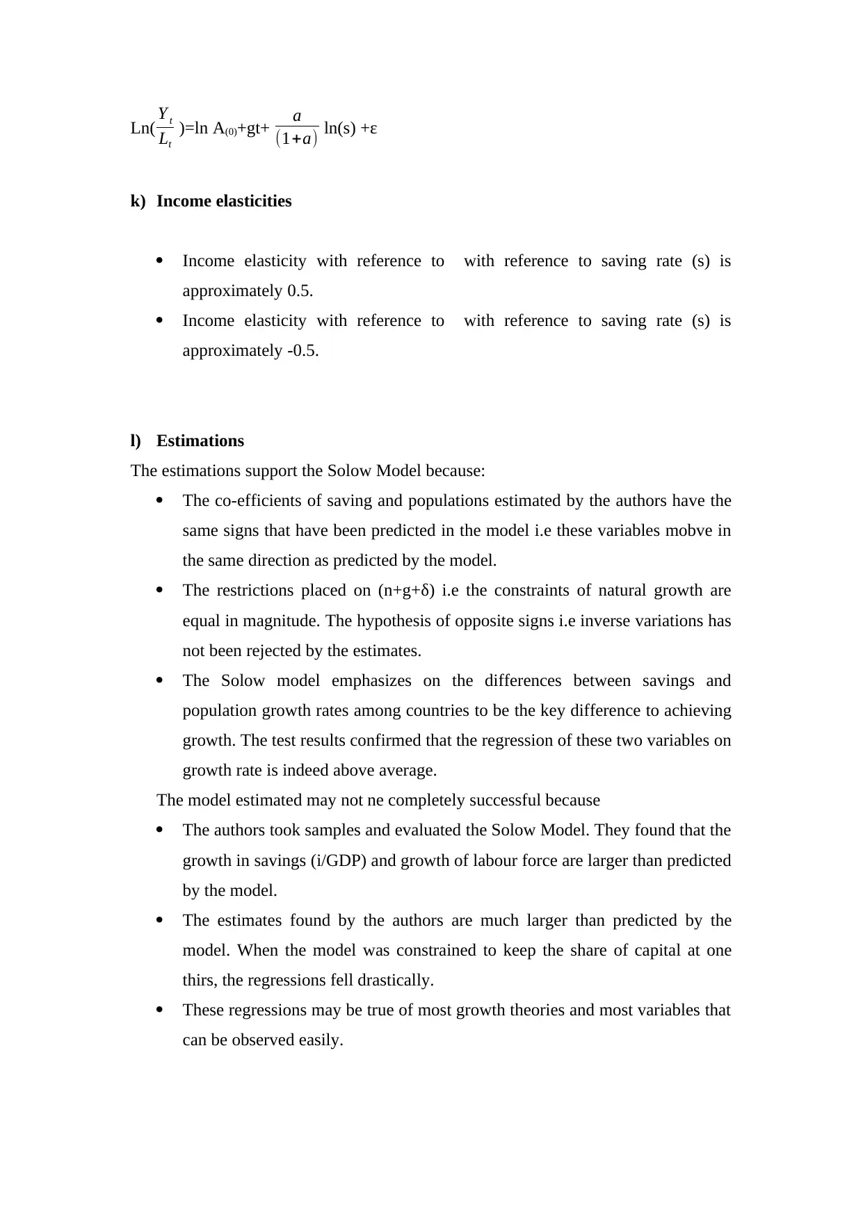
Ln( Y t
Lt
)=ln A(0)+gt+ a
(1+a) ln(s) +ε
k) Income elasticities
Income elasticity with reference to with reference to saving rate (s) is
approximately 0.5.
Income elasticity with reference to with reference to saving rate (s) is
approximately -0.5.
l) Estimations
The estimations support the Solow Model because:
The co-efficients of saving and populations estimated by the authors have the
same signs that have been predicted in the model i.e these variables mobve in
the same direction as predicted by the model.
The restrictions placed on (n+g+δ) i.e the constraints of natural growth are
equal in magnitude. The hypothesis of opposite signs i.e inverse variations has
not been rejected by the estimates.
The Solow model emphasizes on the differences between savings and
population growth rates among countries to be the key difference to achieving
growth. The test results confirmed that the regression of these two variables on
growth rate is indeed above average.
The model estimated may not ne completely successful because
The authors took samples and evaluated the Solow Model. They found that the
growth in savings (i/GDP) and growth of labour force are larger than predicted
by the model.
The estimates found by the authors are much larger than predicted by the
model. When the model was constrained to keep the share of capital at one
thirs, the regressions fell drastically.
These regressions may be true of most growth theories and most variables that
can be observed easily.
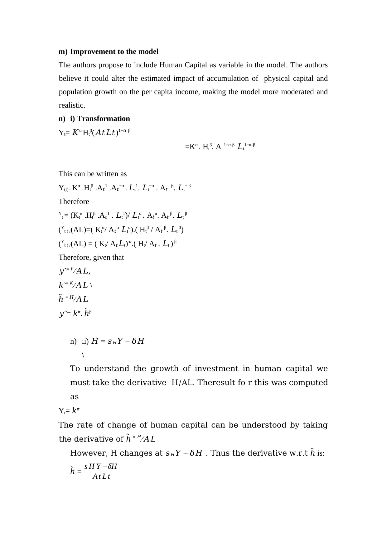
m) Improvement to the model
The authors propose to include Human Capital as variable in the model. The authors
believe it could alter the estimated impact of accumulation of physical capital and
population growth on the per capita income, making the model more moderated and
realistic.
n) i) Transformation
Yt= 𝐾α Htβ(𝐴𝑡𝐿𝑡)1−𝛼-β
=Kα . Htβ. A 1−α-β 𝐿t1−α-β
This can be written as
Y(t)= Kα .Htβ .A𝑡1 .A𝑡−α . 𝐿t1. 𝐿t−α . A𝑡 –β. 𝐿t− β
Therefore
Yt = (Ktα .Htβ .A𝑡1 . 𝐿t1)/ 𝐿tα . A𝑡α. A𝑡 β. 𝐿t β
(Yt ) /(AL)=( Ktα/ A𝑡α 𝐿tα).( Htβ / A𝑡 β. 𝐿t β)
(Yt ) /(AL) = ( Kt/ A𝑡𝐿t) α.( Ht/ A𝑡 . 𝐿t ) β
Therefore, given that
𝑦̃ = 𝑌⁄𝐴𝐿,
𝑘̃ = 𝐾⁄𝐴𝐿 \
ℎ̃ = 𝐻⁄𝐴𝐿
𝑦̃ = 𝑘̃α. ℎ̃β
n) ii) 𝐻̇ = 𝑠𝐻𝑌 – 𝛿𝐻
\
To understand the growth of investment in human capital we
must take the derivative H/AL. Theresult fo r this was computed
as
Yt= 𝑘̃α
The rate of change of human capital can be understood by taking
the derivative of ℎ̃ = 𝐻⁄𝐴𝐿
However, H changes at 𝑠𝐻𝑌 – 𝛿𝐻 . Thus the derivative w.r.t is:ℎ̃
=ℎ̃ s H Y – δH
A t L t
⊘ This is a preview!⊘
Do you want full access?
Subscribe today to unlock all pages.
Trusted by 1+ million students worldwide
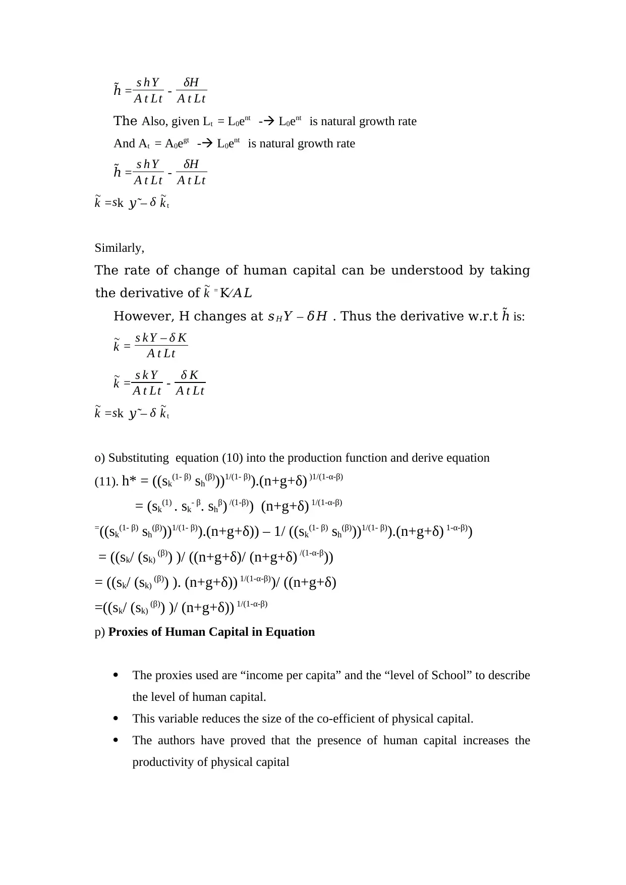
=ℎ̃ s h Y
A t Lt - δH
A t Lt
The Also, given Lt = L0ent - L0ent is natural growth rate
And At = A0egt - L0ent is natural growth rate
=ℎ̃ s h Y
A t Lt - δH
A t Lt
~
k = sk 𝑦̃ – δ ~
k t
Similarly,
The rate of change of human capital can be understood by taking
the derivative of ~
k = K⁄𝐴𝐿
However, H changes at 𝑠𝐻𝑌 – 𝛿𝐻 . Thus the derivative w.r.t is:ℎ̃
~
k = s k Y – δ K
A t Lt
~
k = s k Y
A t Lt - δ K
A t Lt
~
k = sk 𝑦̃ – δ ~
k t
o) Substituting equation (10) into the production function and derive equation
(11). h* = ((sk(1- β) sh(β)))1/(1- β)).(n+g+δ) )1/(1-α-β)
= (sk(1) . sk- β. shβ) /(1-β)) (n+g+δ) 1/(1-α-β)
=((sk(1- β) sh(β)))1/(1- β)).(n+g+δ)) – 1/ ((sk(1- β) sh(β)))1/(1- β)).(n+g+δ) 1-α-β))
= ((sk/ (sk) (β)) )/ ((n+g+δ)/ (n+g+δ) /(1-α-β))
= ((sk/ (sk) (β)) ). (n+g+δ)) 1/(1-α-β))/ ((n+g+δ)
=((sk/ (sk) (β)) )/ (n+g+δ)) 1/(1-α-β)
p) Proxies of Human Capital in Equation
The proxies used are “income per capita” and the “level of School” to describe
the level of human capital.
This variable reduces the size of the co-efficient of physical capital.
The authors have proved that the presence of human capital increases the
productivity of physical capital
A t Lt - δH
A t Lt
The Also, given Lt = L0ent - L0ent is natural growth rate
And At = A0egt - L0ent is natural growth rate
=ℎ̃ s h Y
A t Lt - δH
A t Lt
~
k = sk 𝑦̃ – δ ~
k t
Similarly,
The rate of change of human capital can be understood by taking
the derivative of ~
k = K⁄𝐴𝐿
However, H changes at 𝑠𝐻𝑌 – 𝛿𝐻 . Thus the derivative w.r.t is:ℎ̃
~
k = s k Y – δ K
A t Lt
~
k = s k Y
A t Lt - δ K
A t Lt
~
k = sk 𝑦̃ – δ ~
k t
o) Substituting equation (10) into the production function and derive equation
(11). h* = ((sk(1- β) sh(β)))1/(1- β)).(n+g+δ) )1/(1-α-β)
= (sk(1) . sk- β. shβ) /(1-β)) (n+g+δ) 1/(1-α-β)
=((sk(1- β) sh(β)))1/(1- β)).(n+g+δ)) – 1/ ((sk(1- β) sh(β)))1/(1- β)).(n+g+δ) 1-α-β))
= ((sk/ (sk) (β)) )/ ((n+g+δ)/ (n+g+δ) /(1-α-β))
= ((sk/ (sk) (β)) ). (n+g+δ)) 1/(1-α-β))/ ((n+g+δ)
=((sk/ (sk) (β)) )/ (n+g+δ)) 1/(1-α-β)
p) Proxies of Human Capital in Equation
The proxies used are “income per capita” and the “level of School” to describe
the level of human capital.
This variable reduces the size of the co-efficient of physical capital.
The authors have proved that the presence of human capital increases the
productivity of physical capital
Paraphrase This Document
Need a fresh take? Get an instant paraphrase of this document with our AI Paraphraser

The regressions for better with this equation.
1 out of 11
Related Documents


Your All-in-One AI-Powered Toolkit for Academic Success.
+13062052269
info@desklib.com
Available 24*7 on WhatsApp / Email
![[object Object]](/_next/static/media/star-bottom.7253800d.svg)
Unlock your academic potential
Copyright © 2020–2026 A2Z Services. All Rights Reserved. Developed and managed by ZUCOL.