ECO 578 University Statistics: Fall 2018 Detailed Homework Assignment

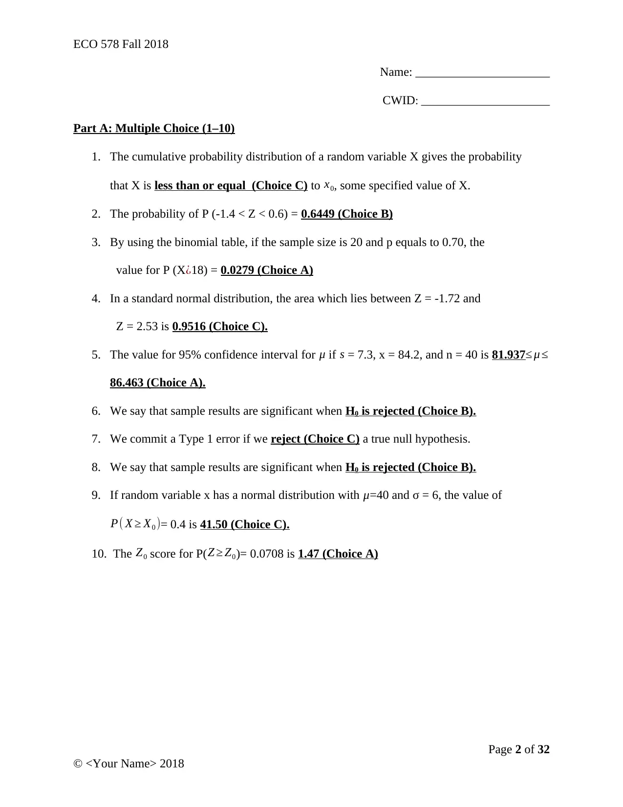
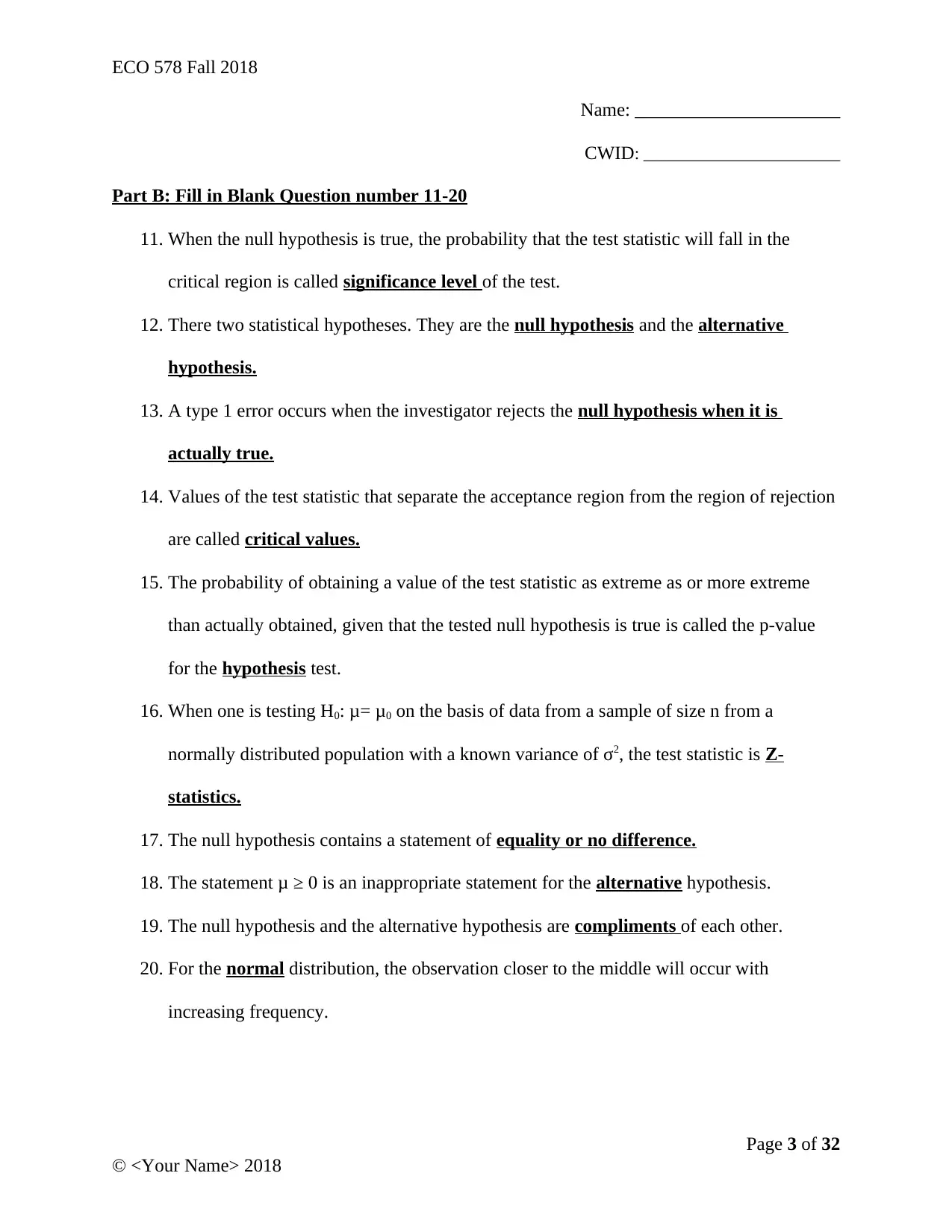
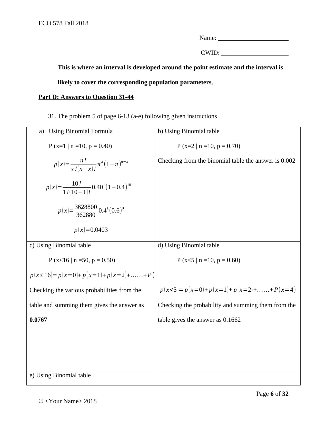
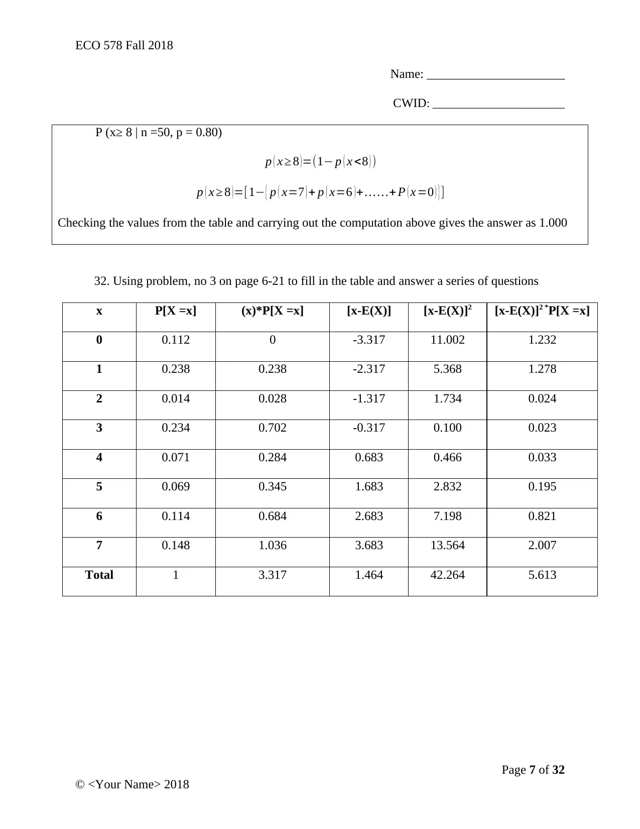
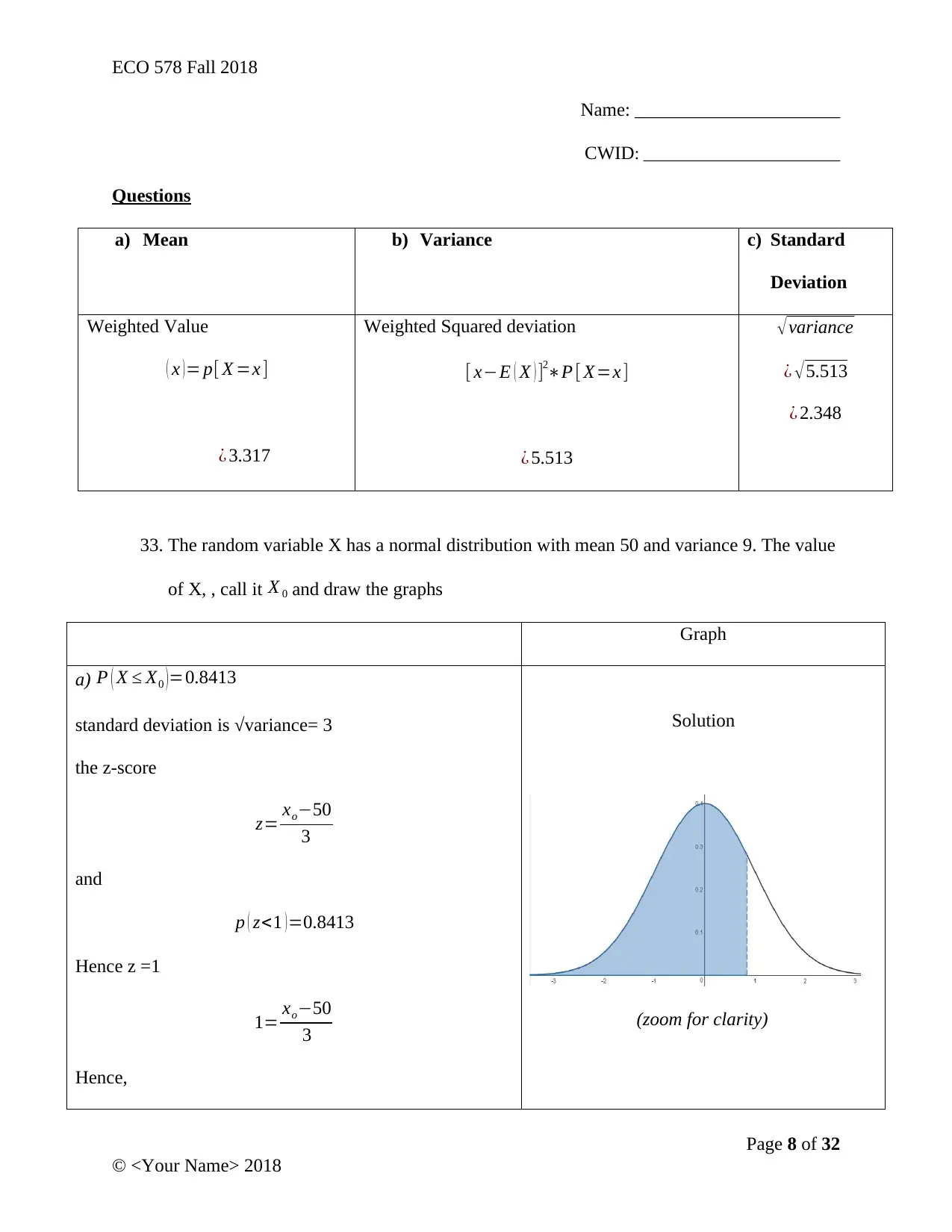
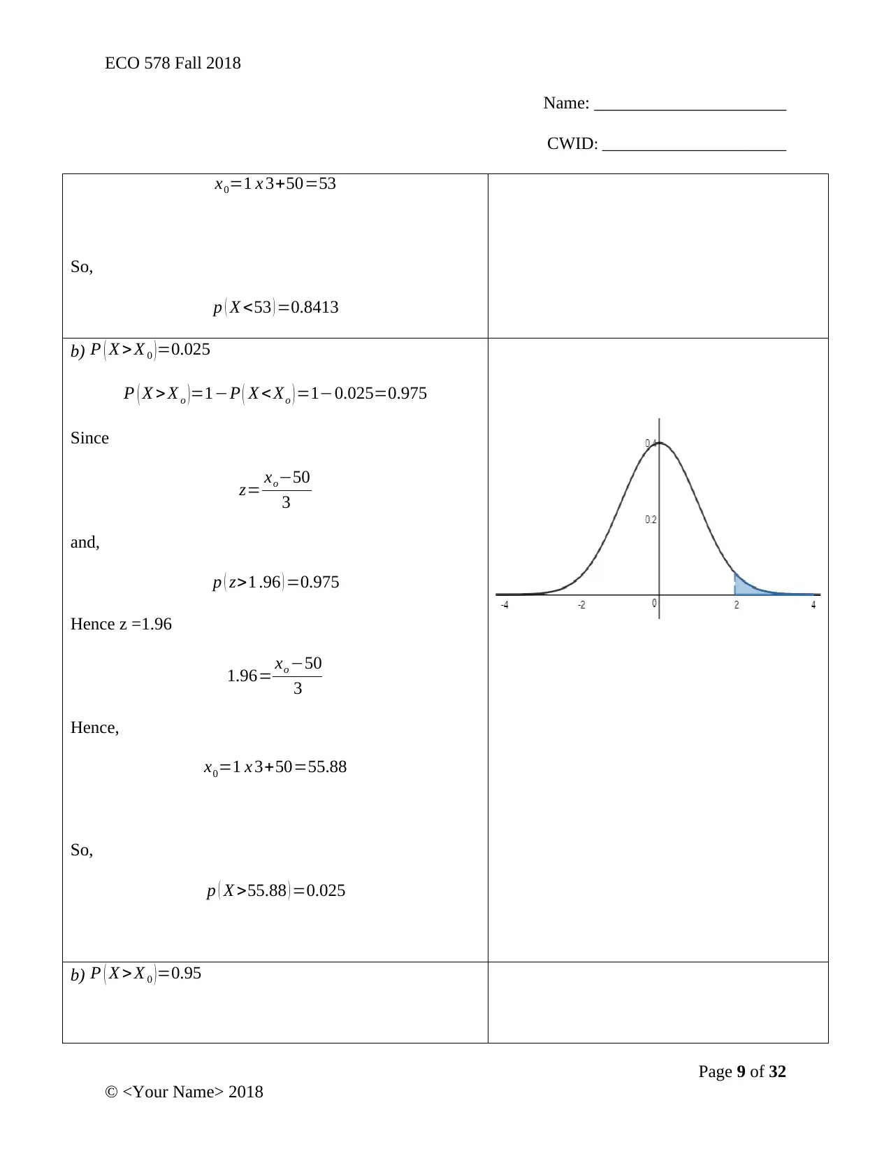
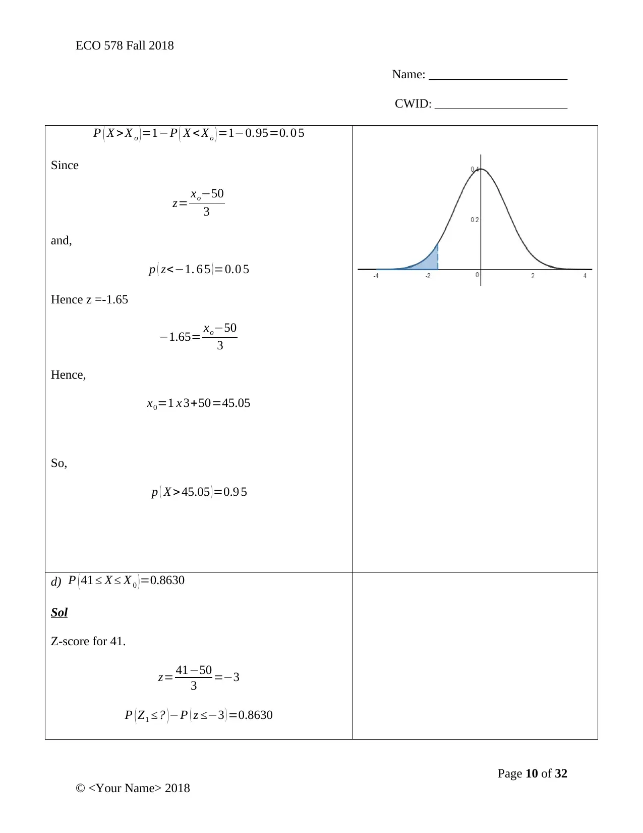
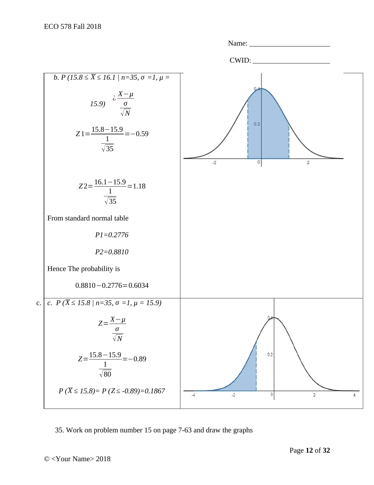
This document provides a comprehensive solution to a statistics homework assignment for ECO 578, Fall 2018. It includes multiple-choice answers covering cumulative probability, standard normal distribution calculations, binomial probabilities, and confidence intervals. The solution also involves fill-in-the-blank questions focusing on hypothesis testing, Type I errors, critical values, and p-values. Furthermore, it addresses conceptual questions related to discrete vs. continuous variables, normal distribution characteristics, Z-test vs. t-test usage, the Q’ method in binomial probability, Type I vs. Type II errors, the Central Limit Theorem, distribution of sample means, null and alternative hypotheses, significance levels, and interval estimates. Finally, the solution provides detailed answers to calculation-based problems involving binomial formulas, probability distributions, normal distributions, and hypothesis testing with accompanying graphs. The problems cover a wide range of statistical concepts and applications.

ECO 578 Fall 2018
Name: ______________________
CWID: _______________________
University
Statistics
By
Your Name
Lecturers Name
Date
Page 1 of 32
© <Your Name> 2018

ECO 578 Fall 2018
Name: ______________________
CWID: _______________________
Part A: Multiple Choice (1–10)
1. The cumulative probability distribution of a random variable X gives the probability
that X is less than or equal (Choice C) to x0, some specified value of X.
2. The probability of P (-1.4 < Z < 0.6) = 0.6449 (Choice B)
3. By using the binomial table, if the sample size is 20 and p equals to 0.70, the
value for P (X¿18) = 0.0279 (Choice A)
4. In a standard normal distribution, the area which lies between Z = -1.72 and
Z = 2.53 is 0.9516 (Choice C).
5. The value for 95% confidence interval for μ if s = 7.3, x = 84.2, and n = 40 is 81.937≤ μ ≤
86.463 (Choice A).
6. We say that sample results are significant when H0 is rejected (Choice B).
7. We commit a Type 1 error if we reject (Choice C) a true null hypothesis.
8. We say that sample results are significant when H0 is rejected (Choice B).
9. If random variable x has a normal distribution with μ=40 and σ = 6, the value of
P( X ≥ X0 )= 0.4 is 41.50 (Choice C).
10. The Z0 score for P( Z ≥ Z0)= 0.0708 is 1.47 (Choice A)
Page 2 of 32
© <Your Name> 2018

ECO 578 Fall 2018
Name: ______________________
CWID: _______________________
Part B: Fill in Blank Question number 11-20
11. When the null hypothesis is true, the probability that the test statistic will fall in the
critical region is called significance level of the test.
12. There two statistical hypotheses. They are the null hypothesis and the alternative
hypothesis.
13. A type 1 error occurs when the investigator rejects the null hypothesis when it is
actually true.
14. Values of the test statistic that separate the acceptance region from the region of rejection
are called critical values.
15. The probability of obtaining a value of the test statistic as extreme as or more extreme
than actually obtained, given that the tested null hypothesis is true is called the p-value
for the hypothesis test.
16. When one is testing H0: μ= μ0 on the basis of data from a sample of size n from a
normally distributed population with a known variance of σ2, the test statistic is Z-
statistics.
17. The null hypothesis contains a statement of equality or no difference.
18. The statement μ ≥ 0 is an inappropriate statement for the alternative hypothesis.
19. The null hypothesis and the alternative hypothesis are compliments of each other.
20. For the normal distribution, the observation closer to the middle will occur with
increasing frequency.
Page 3 of 32
© <Your Name> 2018

ECO 578 Fall 2018
Name: ______________________
CWID: _______________________
PART C: ANSWER THE FOLLOWING QUESTIONS (21-30)
21. The difference between discrete random variable and continuous random variable.
Discrete random variables can only take a finite number of values. Example is the
number of posts used in electrical installation. On the other hand, the continuous
random variable takes values within a given a range or interval. Example is the
height of an individual.
22. Description of the normal distribution.
This is a distribution that gives a bell-shaped curve while giving a description of the
spread of a characteristic throughout a population.
23. When the Z-test should be used and when t-test should be used.
The Z-test should be used when there is a large sample size i.e. n is greater than 30
or when the standard deviation is known for any sample size. On the other hand, t-
test should be used when the sample size is small. i.e. n<30 or when the value of the s
is given or has to be determined.
24. The Q’ method with regards to Binomial Probability.
The Q method in binomial probability involves defining the success for an
individual trial, then the probability of the success is determined. After that, the
probability of failure is determined. The number of trials is defined and finally the
successes number out of the trial (Bruce, 2015).
25. Difference between Type 1 error and Type II error.
A Type I error is an error committed in statistics when the null hypothesis is
rejected but it is true. It is also known as a false positive. On the other hand, a type
Page 4 of 32
© <Your Name> 2018

ECO 578 Fall 2018
Name: ______________________
CWID: _______________________
11 error is committed when we fail to reject the null hypothesis when in real else it is
false. It is also known as a false negative (Hinton, 2014) .
26. The Central Limit Theorem.
According to the central limit theorem, the sampling distribution for any
distribution in statistics is normal or close to normal when the sample size large
enough is selected. The sample size is determined based on the accuracy needed and
the shape of the population under consideration.
27. Distribution sample means.
This refers to the theoretical distribution of values of a sample which the mean of
the sample takes in all the possible sample combinations of given sizes made from
the selected population.
28. The null and alternative hypothesis
The null hypothesis refers to the hypothesis that indicate that the population
parameter is equal to or there is no difference with a given specification. On the
other hand, the alternative hypothesis is the compliment of the null hypothesis and
it indicates non-equality or existence of difference with a given specification.
29. The significance level.
This refers to a value in statistical hypothesis test which indicates the boundary of
the region below which a conclusion can be drawn that a given p-value shows
significant evidence in favor of the alternative hypothesis or against the null
hypothesis.
30. What is Interval Estimate.
Page 5 of 32
© <Your Name> 2018

ECO 578 Fall 2018
Name: ______________________
CWID: _______________________
This is where an interval is developed around the point estimate and the interval is
likely to cover the corresponding population parameters.
Part D: Answers to Question 31-44
31. The problem 5 of page 6-13 (a-e) following given instructions
a) Using Binomial Formula
P (x=1 | n =10, p = 0.40)
p ( x ) = n !
x ! ( n−x ) ! π x (1−π )n−x
p ( x ) = 10 !
1 ! ( 10−1 ) ! 0.401 (1−0.4)10−1
p ( x )=3628800
362880 0.41 (0.6)9
p ( x ) =0.0403
b) Using Binomial table
P (x=2 | n =10, p = 0.70)
Checking from the binomial table the answer is 0.002
c) Using Binomial table
P (x≤16 | n =50, p = 0.50)
p ( x ≤ 16 ) = p ( x=0 ) + p ( x=1 ) + p ( x=2 ) +… …+ P (x=16)
Checking the various probabilities from the
table and summing them gives the answer as
0.0767
d) Using Binomial table
P (x<5 | n =10, p = 0.60)
p ( x<5 ) = p ( x=0 ) + p ( x=1 ) + p ( x=2 ) +… …+ P( x=4)
Checking the probability and summing them from the
table gives the answer as 0.1662
e) Using Binomial table
Page 6 of 32
© <Your Name> 2018

ECO 578 Fall 2018
Name: ______________________
CWID: _______________________
P (x≥ 8 | n =50, p = 0.80)
p ( x ≥ 8 )=(1− p ( x <8 ) )
p ( x ≥ 8 ) =[1− { p ( x=7 ) + p ( x=6 ) + … …+ P ( x =0 ) } ]
Checking the values from the table and carrying out the computation above gives the answer as 1.000
32. Using problem, no 3 on page 6-21 to fill in the table and answer a series of questions
x P[X =x] (x)*P[X =x] [x-E(X)] [x-E(X)]2 [x-E(X)]2 *P[X =x]
0 0.112 0 -3.317 11.002 1.232
1 0.238 0.238 -2.317 5.368 1.278
2 0.014 0.028 -1.317 1.734 0.024
3 0.234 0.702 -0.317 0.100 0.023
4 0.071 0.284 0.683 0.466 0.033
5 0.069 0.345 1.683 2.832 0.195
6 0.114 0.684 2.683 7.198 0.821
7 0.148 1.036 3.683 13.564 2.007
Total 1 3.317 1.464 42.264 5.613
Page 7 of 32
© <Your Name> 2018

ECO 578 Fall 2018
Name: ______________________
CWID: _______________________
Questions
a) Mean b) Variance c) Standard
Deviation
Weighted Value
( x )= p[ X =x ]
¿ 3.317
Weighted Squared deviation
[ x−E ( X ) ]2∗P [ X=x ]
¿ 5.513
√variance
¿ √ 5.513
¿ 2.348
33. The random variable X has a normal distribution with mean 50 and variance 9. The value
of X, , call it X 0 and draw the graphs
Graph
a) P ( X ≤ X0 )=0.8413
standard deviation is √variance= 3
the z-score
z= xo−50
3
and
p ( z<1 ) =0.8413
Hence z =1
1= xo−50
3
Hence,
Solution
(zoom for clarity)
Page 8 of 32
© <Your Name> 2018

ECO 578 Fall 2018
Name: ______________________
CWID: _______________________
x0=1 x 3+50=53
So,
p ( X <53 ) =0.8413
b) P ( X > X 0 )=0.025
P ( X > X o )=1−P ( X < Xo ) =1−0.025=0.975
Since
z= xo−50
3
and,
p ( z>1 .96 ) =0.975
Hence z =1.96
1.96= xo −50
3
Hence,
x0=1 x 3+50=55.88
So,
p ( X >55.88 ) =0.025
b) P ( X > X 0 )=0.95
Page 9 of 32
© <Your Name> 2018

ECO 578 Fall 2018
Name: ______________________
CWID: _______________________
P ( X > X o ) =1−P ( X < Xo ) =1−0.95=0. 0 5
Since
z= xo−50
3
and,
p ( z<−1. 6 5 )=0.0 5
Hence z =-1.65
−1.65= xo−50
3
Hence,
x0=1 x 3+50=45.05
So,
p ( X > 45.05 )=0.9 5
d) P ( 41 ≤ X ≤ X 0 )=0.8630
Sol
Z-score for 41.
z= 41−50
3 =−3
P ( Z1 ≤? ) −P ( z ≤−3 ) =0.8630
Page 10 of 32
© <Your Name> 2018

ECO 578 Fall 2018
Name: ______________________
CWID: _______________________
p ( z1 ≤ ? ) −0.0013=0.8680
p ( z1 ≤ ? ) =0.8680+0.0013=0.8643
From the z-table
p ( z1 ≤ 1.01 )=0.8643
Hence Z1=1.01
z= xo−50
3 =1.01
xo=53.03
34. The problem no 10 on page 7-63 and the resulting graphs
a. Graphs
b. a. P ( X > 15.95 | n=80, σ =1, μ =15.9)
Z= X−μ
σ
√ N
Z=15.95−15.9
1
√ 80
=0.447
P ( X > 15.95)= P ( Z> 0.447)=0.3274
Page 11 of 32
© <Your Name> 2018

ECO 578 Fall 2018
Name: ______________________
CWID: _______________________
b. P (15.8 ≤ X ≤ 16.1 | n=35, σ =1, μ =
15.9) ¿ X−μ
σ
√N
Z 1= 15.8−15.9
1
√ 35
=−0.59
Z 2= 16.1−15.9
1
√ 35
=1.18
From standard normal table
P1=0.2776
P2=0.8810
Hence The probability is
0.8810−0.2776=0.6034
c. c. P ( X ≤ 15.8 | n=35, σ =1, μ = 15.9)
Z= X−μ
σ
√ N
Z=15.8−15.9
1
√ 80
=−0.89
P ( X ≤ 15.8)= P ( Z ≤ -0.89)=0.1867
35. Work on problem number 15 on page 7-63 and draw the graphs
Page 12 of 32
© <Your Name> 2018