Econ 262 Problem Set 2: Analyzing Worker Salaries with Regression

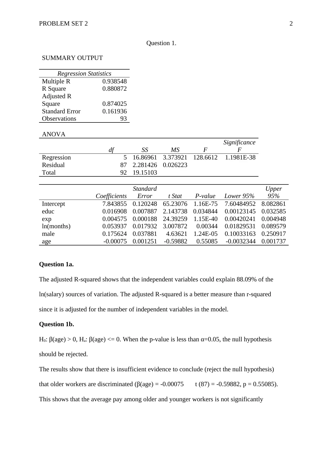
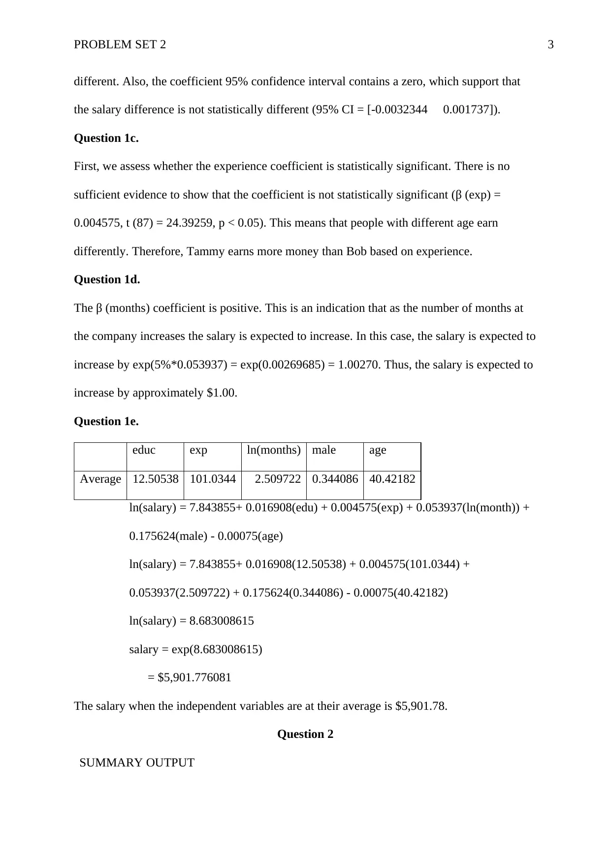
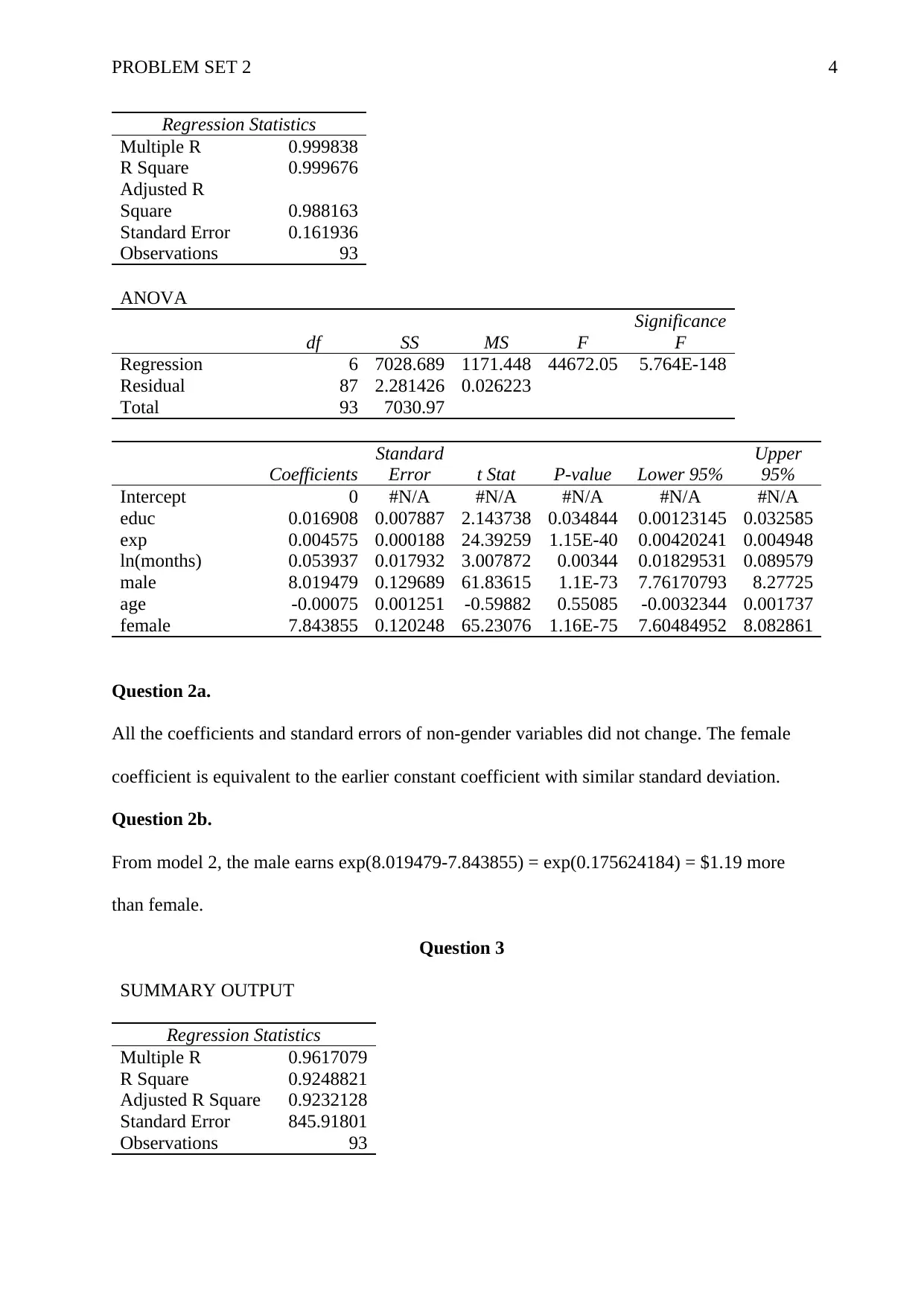
This document presents a solution to Econ 262 Problem Set 2, focusing on the analysis of worker salaries using regression techniques. The assignment involves estimating a regression equation to explain the natural logarithm of salary based on worker characteristics such as education, prior experience, the natural logarithm of months at the company, age, and gender. The solution includes the regression output, interpretation of the adjusted R-squared, and a t-test to assess potential age discrimination. The analysis further investigates the statistical significance of experience on salary and determines the expected salary increase with increased months at the company. Additionally, the document provides calculations of salary based on average independent variable values and extends the analysis to include the impact of gender. Finally, the solution addresses a quadratic relationship between salary and experience. The analysis is based on data from a software firm, considering factors like education, experience, months at the company, age, and gender to understand their influence on monthly salary.

Running head: PROBLEM SET 2 1
Econ 262 Problem Set 2
Name:
Institution:

PROBLEM SET 2 2
Question 1.
SUMMARY OUTPUT
Regression Statistics
Multiple R 0.938548
R Square 0.880872
Adjusted R
Square 0.874025
Standard Error 0.161936
Observations 93
ANOVA
df SS MS F
Significance
F
Regression 5 16.86961 3.373921 128.6612 1.1981E-38
Residual 87 2.281426 0.026223
Total 92 19.15103
Coefficients
Standard
Error t Stat P-value Lower 95%
Upper
95%
Intercept 7.843855 0.120248 65.23076 1.16E-75 7.60484952 8.082861
educ 0.016908 0.007887 2.143738 0.034844 0.00123145 0.032585
exp 0.004575 0.000188 24.39259 1.15E-40 0.00420241 0.004948
ln(months) 0.053937 0.017932 3.007872 0.00344 0.01829531 0.089579
male 0.175624 0.037881 4.63621 1.24E-05 0.10033163 0.250917
age -0.00075 0.001251 -0.59882 0.55085 -0.0032344 0.001737
Question 1a.
The adjusted R-squared shows that the independent variables could explain 88.09% of the
ln(salary) sources of variation. The adjusted R-squared is a better measure than r-squared
since it is adjusted for the number of independent variables in the model.
Question 1b.
H0: β(age) > 0, Ha: β(age) <= 0. When the p-value is less than α=0.05, the null hypothesis
should be rejected.
The results show that there is insufficient evidence to conclude (reject the null hypothesis)
that older workers are discriminated (β(age) = -0.00075 t (87) = -0.59882, p = 0.55085).
This shows that the average pay among older and younger workers is not significantly

PROBLEM SET 2 3
different. Also, the coefficient 95% confidence interval contains a zero, which support that
the salary difference is not statistically different (95% CI = [-0.0032344 0.001737]).
Question 1c.
First, we assess whether the experience coefficient is statistically significant. There is no
sufficient evidence to show that the coefficient is not statistically significant (β (exp) =
0.004575, t (87) = 24.39259, p < 0.05). This means that people with different age earn
differently. Therefore, Tammy earns more money than Bob based on experience.
Question 1d.
The β (months) coefficient is positive. This is an indication that as the number of months at
the company increases the salary is expected to increase. In this case, the salary is expected to
increase by exp(5%*0.053937) = exp(0.00269685) = 1.00270. Thus, the salary is expected to
increase by approximately $1.00.
Question 1e.
educ exp ln(months) male age
Average 12.50538 101.0344 2.509722 0.344086 40.42182
ln(salary) = 7.843855+ 0.016908(edu) + 0.004575(exp) + 0.053937(ln(month)) +
0.175624(male) - 0.00075(age)
ln(salary) = 7.843855+ 0.016908(12.50538) + 0.004575(101.0344) +
0.053937(2.509722) + 0.175624(0.344086) - 0.00075(40.42182)
ln(salary) = 8.683008615
salary = exp(8.683008615)
= $5,901.776081
The salary when the independent variables are at their average is $5,901.78.
Question 2
SUMMARY OUTPUT

PROBLEM SET 2 4
Regression Statistics
Multiple R 0.999838
R Square 0.999676
Adjusted R
Square 0.988163
Standard Error 0.161936
Observations 93
ANOVA
df SS MS F
Significance
F
Regression 6 7028.689 1171.448 44672.05 5.764E-148
Residual 87 2.281426 0.026223
Total 93 7030.97
Coefficients
Standard
Error t Stat P-value Lower 95%
Upper
95%
Intercept 0 #N/A #N/A #N/A #N/A #N/A
educ 0.016908 0.007887 2.143738 0.034844 0.00123145 0.032585
exp 0.004575 0.000188 24.39259 1.15E-40 0.00420241 0.004948
ln(months) 0.053937 0.017932 3.007872 0.00344 0.01829531 0.089579
male 8.019479 0.129689 61.83615 1.1E-73 7.76170793 8.27725
age -0.00075 0.001251 -0.59882 0.55085 -0.0032344 0.001737
female 7.843855 0.120248 65.23076 1.16E-75 7.60484952 8.082861
Question 2a.
All the coefficients and standard errors of non-gender variables did not change. The female
coefficient is equivalent to the earlier constant coefficient with similar standard deviation.
Question 2b.
From model 2, the male earns exp(8.019479-7.843855) = exp(0.175624184) = $1.19 more
than female.
Question 3
SUMMARY OUTPUT
Regression Statistics
Multiple R 0.9617079
R Square 0.9248821
Adjusted R Square 0.9232128
Standard Error 845.91801
Observations 93

PROBLEM SET 2 5
ANOVA
df SS MS F
Significance
F
Regression 2 7.93E+08 396471250 554.0579 2.56E-51
Residual 90 64401955 715577.275
Total 92 8.57E+08
Coefficients
Standard
Error t Stat P-value Lower 95%
Upper
95%
Intercept 3251.8764 176.1852 18.4571529 2.39E-32 2901.854 3601.899
exp 32.856708 3.021915 10.8728092 4.47E-18 26.85315 38.86027
exp^2 -0.0017898 0.009358 -0.1912559 0.848756 -0.02038 0.016802
Question 3a.
The minimum salary has been called-out and is 1,895.00 and the maximum salary is
16,247.00.
Question 3b.
The regression analysis shows that the coefficient of exp^2 is not statistically significant (β
(exp^2) = -0.0017898, t (90) = -0.1912559, p-value = 0.848756). Therefore, it can be

PROBLEM SET 2 6
concluded that there is no significant quadratic linear relationship between salary and
experience.