ECON6000: Demand Forecasting and Analysis for Schmeckt Gut Report
VerifiedAdded on 2023/05/28
|16
|3796
|493
Report
AI Summary
This report, directed to the board members of Schmeckt Gut, analyzes the demand for a new product using data from the company's research department. It employs regression analysis to understand the influence of variables such as consumer income, inflation, and tariff rates, projecting demand under four different scenarios. The analysis reveals that income growth is the most significant factor impacting demand, although the nature of the impact varies across scenarios. The report provides detailed regression outputs, discussing the relationships between variables like income, tariffs, inflation, and the number of stores. The findings highlight the importance of considering economic principles, such as the Laffer curve and Phillips curve, in forecasting demand. The report concludes with strategic recommendations for the board based on the different projected scenarios, emphasizing the need for a thorough understanding of economic factors to effectively launch the new product.

1
ECON6000 ECONOMIC PRINCIPLES & DECISION MAKING
ASSESSMENT 3
ECON6000 ECONOMIC PRINCIPLES & DECISION MAKING
ASSESSMENT 3
Paraphrase This Document
Need a fresh take? Get an instant paraphrase of this document with our AI Paraphraser
2
Executive summary
This is a report directed to the board member of Schmeckt Gut regarding the demand for the
new product of the company. The demand forecasting before the launch of the product is
important for the strategy formulation and decision making. The objective of this paper is to
analyse the data provided by the research department of the company to understand the
variables that influence the demand for the product. The study divides the projection into four
different scenarios and regression analysis is done based on the data. The study finds out that,
income growth of the consumer is the most important variable that impacts the demand for
the new product. However, the nature of the impact on the demand depends on the projection
of the variables. The study also recommends strategies to the board members based on the
different scenarios.
3
Table of contents
Introduction................................................................................................................................4
Methods......................................................................................................................................4
Discussion..................................................................................................................................4
Recommendation......................................................................................................................10
Conclusion................................................................................................................................11
Reference..................................................................................................................................13
⊘ This is a preview!⊘
Do you want full access?
Subscribe today to unlock all pages.
Trusted by 1+ million students worldwide
4
Introduction
According to the principle of economics, the demand for a product depends on a lot of direct
and indirect factors. It is important for a company like Schmeckt Gut to understand and
forecast the demand for their new product. The income of the consumers, inflation and the
tariff rate has a crucial influence on the demand of the product. The objective of this report is
to understand the influence of the variables such as the change in the income, inflation and
the tariff rate.
Methods
The study uses the data of the research department of the company and uses regression
analysis to synthesise the data in order to get an insight regarding the demand for the new
product of the company.
Discussion
Different projections regarding the variable
Scenario 1- 5% increase in income, 10% tariff rate and 5% inflation
This scenario is possible as high-income growth of 5% with the presence of a 10% tariff rate
can change the demand for the product in the domestic market. In this case, the demand curve
shifts to the right and increases the price of the product. This in turn, also increases the
inflation level in the economy. Boserup (2017) stated that this is a common phenomenon
under the boom phase of the business cycle to have a higher inflation level corresponding to a
higher income of the consumer. In addition to that, the increased consumption corresponding
to the increased income can also increase the overall output of the economy as per the theory
of aggregate demand. In both the ways, the price of the product has the opportunity to go up
pushing a lot of pressure on the inflation of the economy (Pigou, 2017). Furthermore, this
scenario also has a high tariff rate which can be considered as a tax for the importer. Laffer
curve shows that, with the increase in the tax rate, the revenue of the government increases as
people prefer to buy from outside with the tariff rate applied. However, after a certain point,
the consumers prefer to buy the products from the domestic market as the tariff rate increase
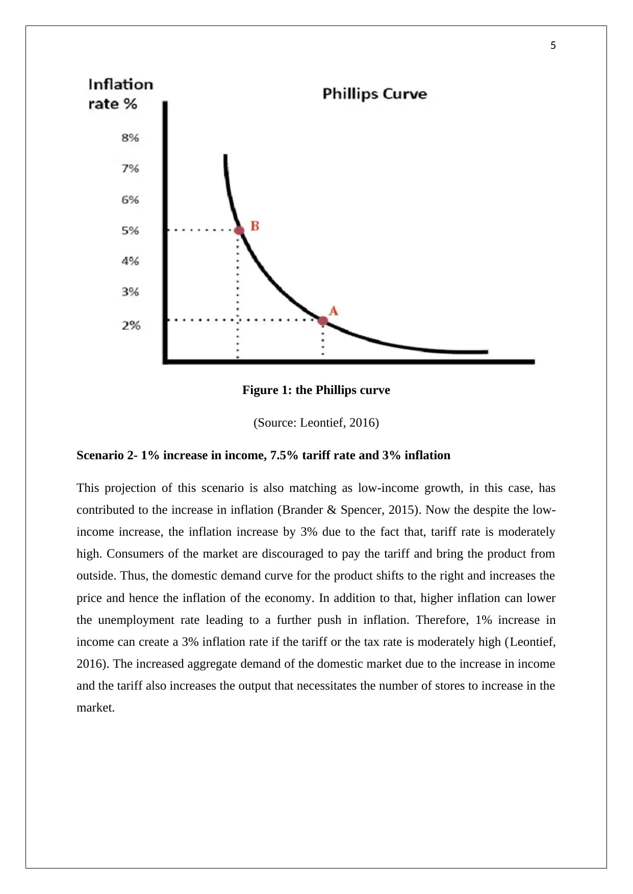
further. Lastly, as per the theory of Phillips as the income increases the number of
unemployed people decreases that impacts on the inflation rate and the number of stores in
the market.
Introduction
According to the principle of economics, the demand for a product depends on a lot of direct
and indirect factors. It is important for a company like Schmeckt Gut to understand and
forecast the demand for their new product. The income of the consumers, inflation and the
tariff rate has a crucial influence on the demand of the product. The objective of this report is
to understand the influence of the variables such as the change in the income, inflation and
the tariff rate.
Methods
The study uses the data of the research department of the company and uses regression
analysis to synthesise the data in order to get an insight regarding the demand for the new
product of the company.
Discussion
Different projections regarding the variable
Scenario 1- 5% increase in income, 10% tariff rate and 5% inflation
This scenario is possible as high-income growth of 5% with the presence of a 10% tariff rate
can change the demand for the product in the domestic market. In this case, the demand curve
shifts to the right and increases the price of the product. This in turn, also increases the
inflation level in the economy. Boserup (2017) stated that this is a common phenomenon
under the boom phase of the business cycle to have a higher inflation level corresponding to a
higher income of the consumer. In addition to that, the increased consumption corresponding
to the increased income can also increase the overall output of the economy as per the theory
of aggregate demand. In both the ways, the price of the product has the opportunity to go up
pushing a lot of pressure on the inflation of the economy (Pigou, 2017). Furthermore, this
scenario also has a high tariff rate which can be considered as a tax for the importer. Laffer
curve shows that, with the increase in the tax rate, the revenue of the government increases as
people prefer to buy from outside with the tariff rate applied. However, after a certain point,
the consumers prefer to buy the products from the domestic market as the tariff rate increase
further. Lastly, as per the theory of Phillips as the income increases the number of
unemployed people decreases that impacts on the inflation rate and the number of stores in
the market.
Paraphrase This Document
Need a fresh take? Get an instant paraphrase of this document with our AI Paraphraser
5
Figure 1: the Phillips curve
(Source: Leontief, 2016)
Scenario 2- 1% increase in income, 7.5% tariff rate and 3% inflation
This projection of this scenario is also matching as low-income growth, in this case, has
contributed to the increase in inflation (Brander & Spencer, 2015). Now the despite the low-
income increase, the inflation increase by 3% due to the fact that, tariff rate is moderately
high. Consumers of the market are discouraged to pay the tariff and bring the product from
outside. Thus, the domestic demand curve for the product shifts to the right and increases the
price and hence the inflation of the economy. In addition to that, higher inflation can lower
the unemployment rate leading to a further push in inflation. Therefore, 1% increase in
income can create a 3% inflation rate if the tariff or the tax rate is moderately high (Leontief,
2016). The increased aggregate demand of the domestic market due to the increase in income
and the tariff also increases the output that necessitates the number of stores to increase in the
market.
6
Figure 2: The demand and supply curve
(Source: Chang & Li, 2018)
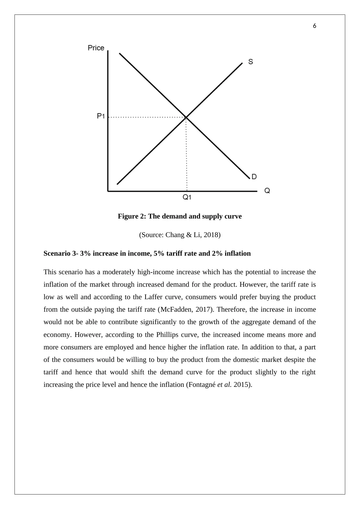
Scenario 3- 3% increase in income, 5% tariff rate and 2% inflation
This scenario has a moderately high-income increase which has the potential to increase the
inflation of the market through increased demand for the product. However, the tariff rate is
low as well and according to the Laffer curve, consumers would prefer buying the product
from the outside paying the tariff rate (McFadden, 2017). Therefore, the increase in income
would not be able to contribute significantly to the growth of the aggregate demand of the
economy. However, according to the Phillips curve, the increased income means more and
more consumers are employed and hence higher the inflation rate. In addition to that, a part
of the consumers would be willing to buy the product from the domestic market despite the
tariff and hence that would shift the demand curve for the product slightly to the right
increasing the price level and hence the inflation (Fontagné et al. 2015).
Figure 2: The demand and supply curve
(Source: Chang & Li, 2018)
Scenario 3- 3% increase in income, 5% tariff rate and 2% inflation
This scenario has a moderately high-income increase which has the potential to increase the
inflation of the market through increased demand for the product. However, the tariff rate is
low as well and according to the Laffer curve, consumers would prefer buying the product
from the outside paying the tariff rate (McFadden, 2017). Therefore, the increase in income
would not be able to contribute significantly to the growth of the aggregate demand of the
economy. However, according to the Phillips curve, the increased income means more and
more consumers are employed and hence higher the inflation rate. In addition to that, a part
of the consumers would be willing to buy the product from the domestic market despite the
tariff and hence that would shift the demand curve for the product slightly to the right
increasing the price level and hence the inflation (Fontagné et al. 2015).
⊘ This is a preview!⊘
Do you want full access?
Subscribe today to unlock all pages.
Trusted by 1+ million students worldwide
7
Figure 3: the aggregate demand and supply curve
(Source: Manganaro, Lawal & Goodall, 2015)
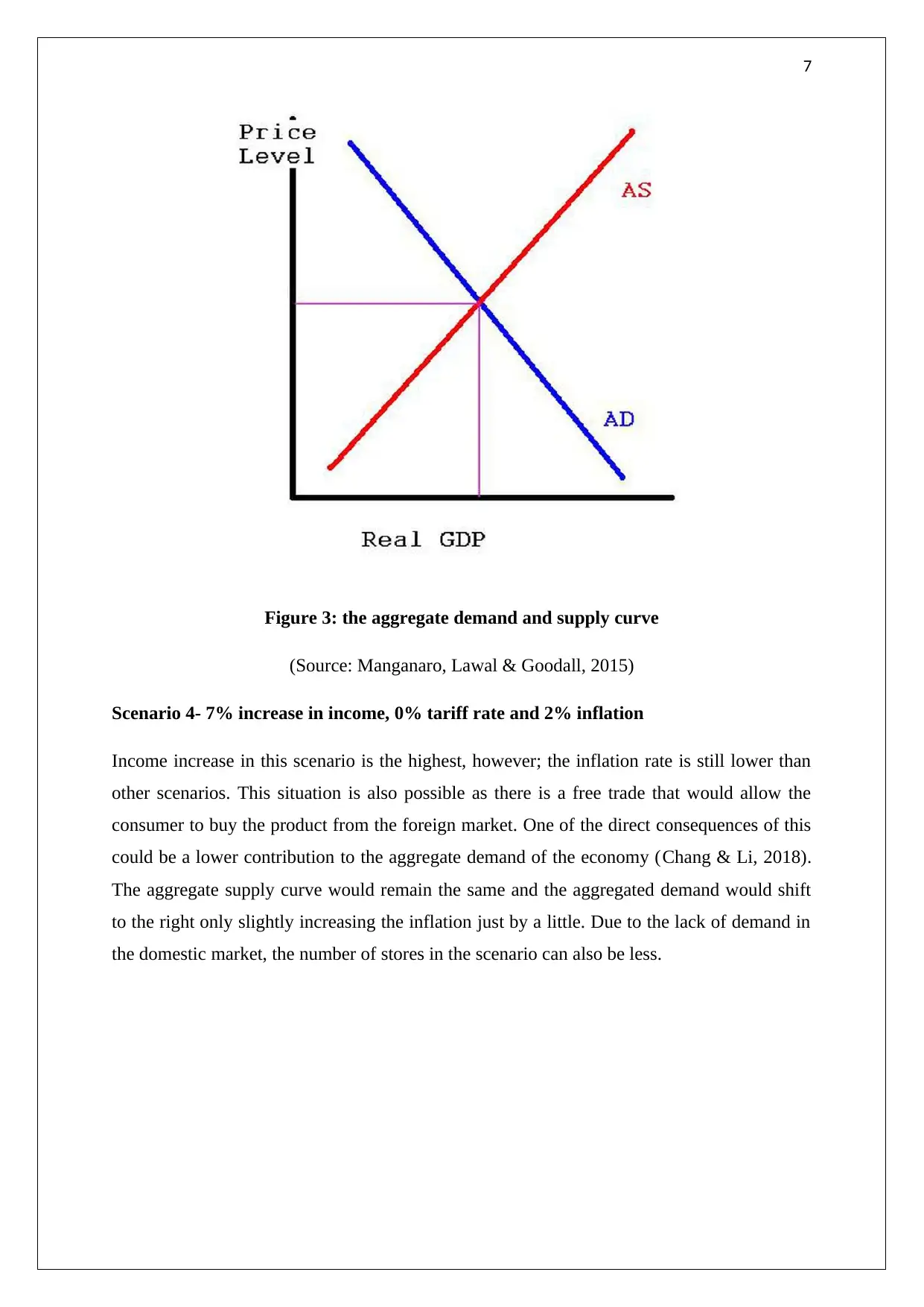
Scenario 4- 7% increase in income, 0% tariff rate and 2% inflation
Income increase in this scenario is the highest, however; the inflation rate is still lower than
other scenarios. This situation is also possible as there is a free trade that would allow the
consumer to buy the product from the foreign market. One of the direct consequences of this
could be a lower contribution to the aggregate demand of the economy (Chang & Li, 2018).
The aggregate supply curve would remain the same and the aggregated demand would shift
to the right only slightly increasing the inflation just by a little. Due to the lack of demand in
the domestic market, the number of stores in the scenario can also be less.
Figure 3: the aggregate demand and supply curve
(Source: Manganaro, Lawal & Goodall, 2015)
Scenario 4- 7% increase in income, 0% tariff rate and 2% inflation
Income increase in this scenario is the highest, however; the inflation rate is still lower than
other scenarios. This situation is also possible as there is a free trade that would allow the
consumer to buy the product from the foreign market. One of the direct consequences of this
could be a lower contribution to the aggregate demand of the economy (Chang & Li, 2018).
The aggregate supply curve would remain the same and the aggregated demand would shift
to the right only slightly increasing the inflation just by a little. Due to the lack of demand in
the domestic market, the number of stores in the scenario can also be less.
Paraphrase This Document
Need a fresh take? Get an instant paraphrase of this document with our AI Paraphraser
8
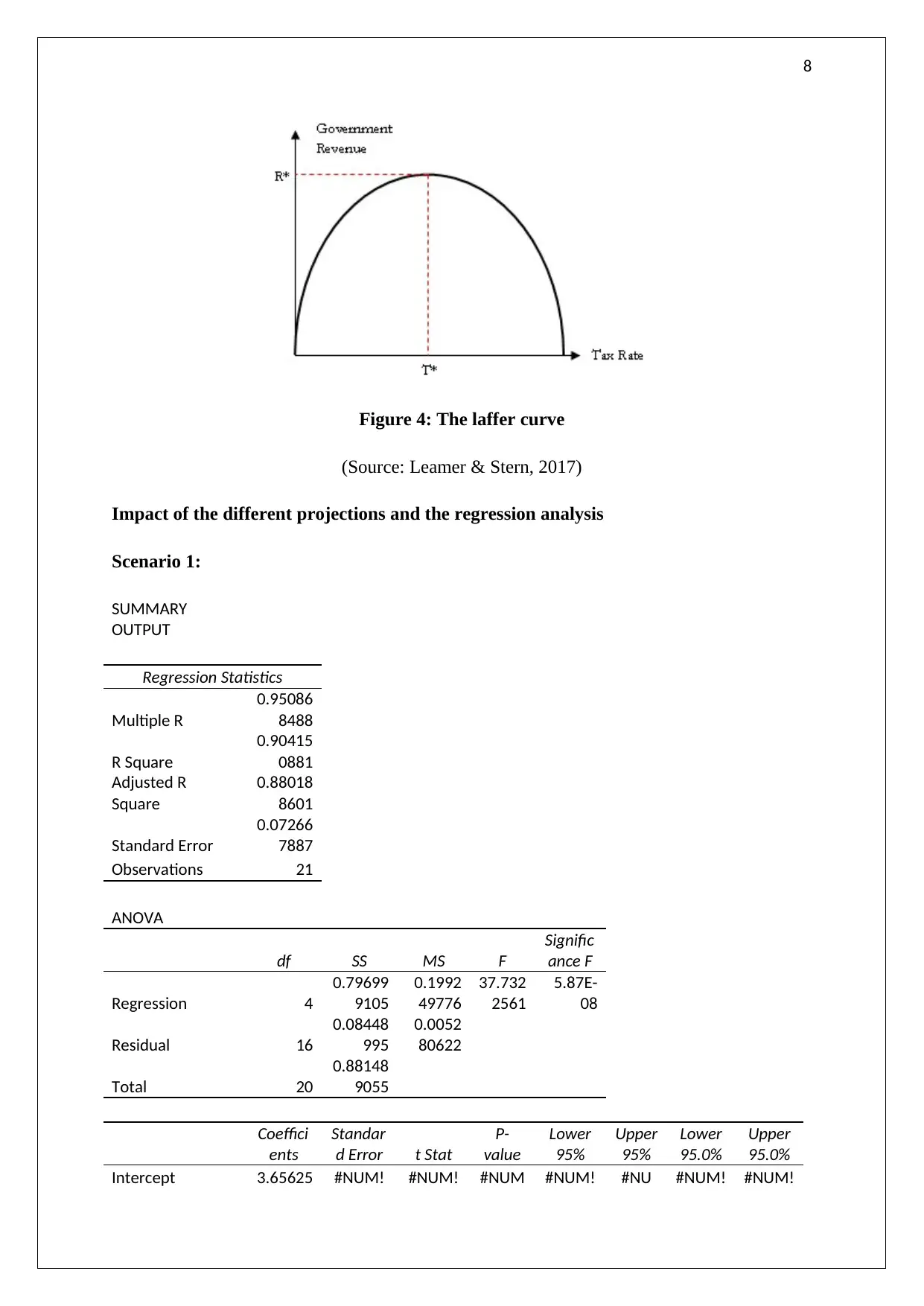
Figure 4: The laffer curve
(Source: Leamer & Stern, 2017)
Impact of the different projections and the regression analysis
Scenario 1:
SUMMARY
OUTPUT
Regression Statistics
Multiple R
0.95086
8488
R Square
0.90415
0881
Adjusted R
Square
0.88018
8601
Standard Error
0.07266
7887
Observations 21
ANOVA
df SS MS F
Signific
ance F
Regression 4
0.79699
9105
0.1992
49776
37.732
2561
5.87E-
08
Residual 16
0.08448
995
0.0052
80622
Total 20
0.88148
9055
Coeffici
ents
Standar
d Error t Stat
P-
value
Lower
95%
Upper
95%
Lower
95.0%
Upper
95.0%
Intercept 3.65625 #NUM! #NUM! #NUM #NUM! #NU #NUM! #NUM!
9
! M!
Number of stores
0.03498
3162
0.01771
1161
1.9752
04351
0.0657
5708
-
0.0025
6
0.072
529
-
0.0025
6
0.0725
29
Changes in the
average income
2.36216
E+11
2.1676E
+11
1.0897
56719
0.2919
6162
-
2.2E+1
1
6.96E
+11
-
2.2E+1
1
6.96E+
11
Changes in tarriff
-
0.54131
7108
0.09743
8961
-
5.5554
4828
4.3483
E-05
-
0.7478
8
-
0.334
76
-
0.7478
8
-
0.3347
6
Inflation
-
124323
99665
114084
17538
-
1.0897
56719
0.2919
6162
-
3.7E+1
0
1.18E
+10
-
3.7E+1
0
1.18E+
10
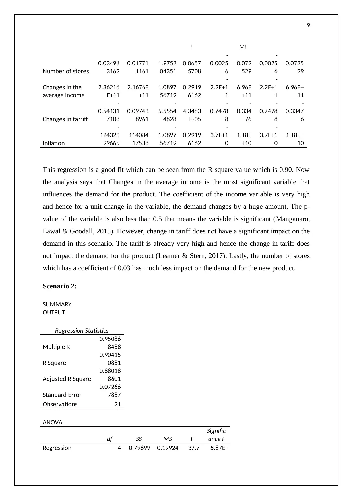
This regression is a good fit which can be seen from the R square value which is 0.90. Now
the analysis says that Changes in the average income is the most significant variable that
influences the demand for the product. The coefficient of the income variable is very high
and hence for a unit change in the variable, the demand changes by a huge amount. The p-
value of the variable is also less than 0.5 that means the variable is significant (Manganaro,
Lawal & Goodall, 2015). However, change in tariff does not have a significant impact on the
demand in this scenario. The tariff is already very high and hence the change in tariff does
not impact the demand for the product (Leamer & Stern, 2017). Lastly, the number of stores
which has a coefficient of 0.03 has much less impact on the demand for the new product.
Scenario 2:
SUMMARY
OUTPUT
Regression Statistics
Multiple R
0.95086
8488
R Square
0.90415
0881
Adjusted R Square
0.88018
8601
Standard Error
0.07266
7887
Observations 21
ANOVA
df SS MS F
Signific
ance F
Regression 4 0.79699 0.19924 37.7 5.87E-
! M!
Number of stores
0.03498
3162
0.01771
1161
1.9752
04351
0.0657
5708
-
0.0025
6
0.072
529
-
0.0025
6
0.0725
29
Changes in the
average income
2.36216
E+11
2.1676E
+11
1.0897
56719
0.2919
6162
-
2.2E+1
1
6.96E
+11
-
2.2E+1
1
6.96E+
11
Changes in tarriff
-
0.54131
7108
0.09743
8961
-
5.5554
4828
4.3483
E-05
-
0.7478
8
-
0.334
76
-
0.7478
8
-
0.3347
6
Inflation
-
124323
99665
114084
17538
-
1.0897
56719
0.2919
6162
-
3.7E+1
0
1.18E
+10
-
3.7E+1
0
1.18E+
10
This regression is a good fit which can be seen from the R square value which is 0.90. Now
the analysis says that Changes in the average income is the most significant variable that
influences the demand for the product. The coefficient of the income variable is very high
and hence for a unit change in the variable, the demand changes by a huge amount. The p-
value of the variable is also less than 0.5 that means the variable is significant (Manganaro,
Lawal & Goodall, 2015). However, change in tariff does not have a significant impact on the
demand in this scenario. The tariff is already very high and hence the change in tariff does
not impact the demand for the product (Leamer & Stern, 2017). Lastly, the number of stores
which has a coefficient of 0.03 has much less impact on the demand for the new product.
Scenario 2:
SUMMARY
OUTPUT
Regression Statistics
Multiple R
0.95086
8488
R Square
0.90415
0881
Adjusted R Square
0.88018
8601
Standard Error
0.07266
7887
Observations 21
ANOVA
df SS MS F
Signific
ance F
Regression 4 0.79699 0.19924 37.7 5.87E-
⊘ This is a preview!⊘
Do you want full access?
Subscribe today to unlock all pages.
Trusted by 1+ million students worldwide
10
9105 9776 3226 08
Residual 16
0.08448
995
0.00528
0622
Total 20
0.88148
9055
Coefficie
nts
Standar
d Error t Stat
P-
value
Lower
95%
Upper
95%
Lower
95.0%
Upper
95.0%
Intercept 3.65625 #NUM! #NUM!
#NU
M! #NUM!
#NU
M! #NUM! #NUM!
Number of stores
0.03498
3162
0.01771
1161
1.97520
4351
0.06
5757
-
0.0025
6
0.072
529
-
0.0025
6
0.0725
29
Changes in the
average income
2.36216
E+11
2.1676E
+11
1.08975
6719
0.29
1962
-
2.2E+1
1
6.96E
+11
-
2.2E+1
1
6.96E+
11
Changes in tarriff
-
0.54131
7108
0.09743
8961
-
5.55544
828
4.35
E-05
-
0.7478
8
-
0.334
76
-
0.7478
8
-
0.3347
6
Inflation
-
124323
99665
114084
17538
-
1.08975
6719
0.29
1962
-
3.7E+1
0
1.18E
+10
-
3.7E+1
0
1.18E+
10
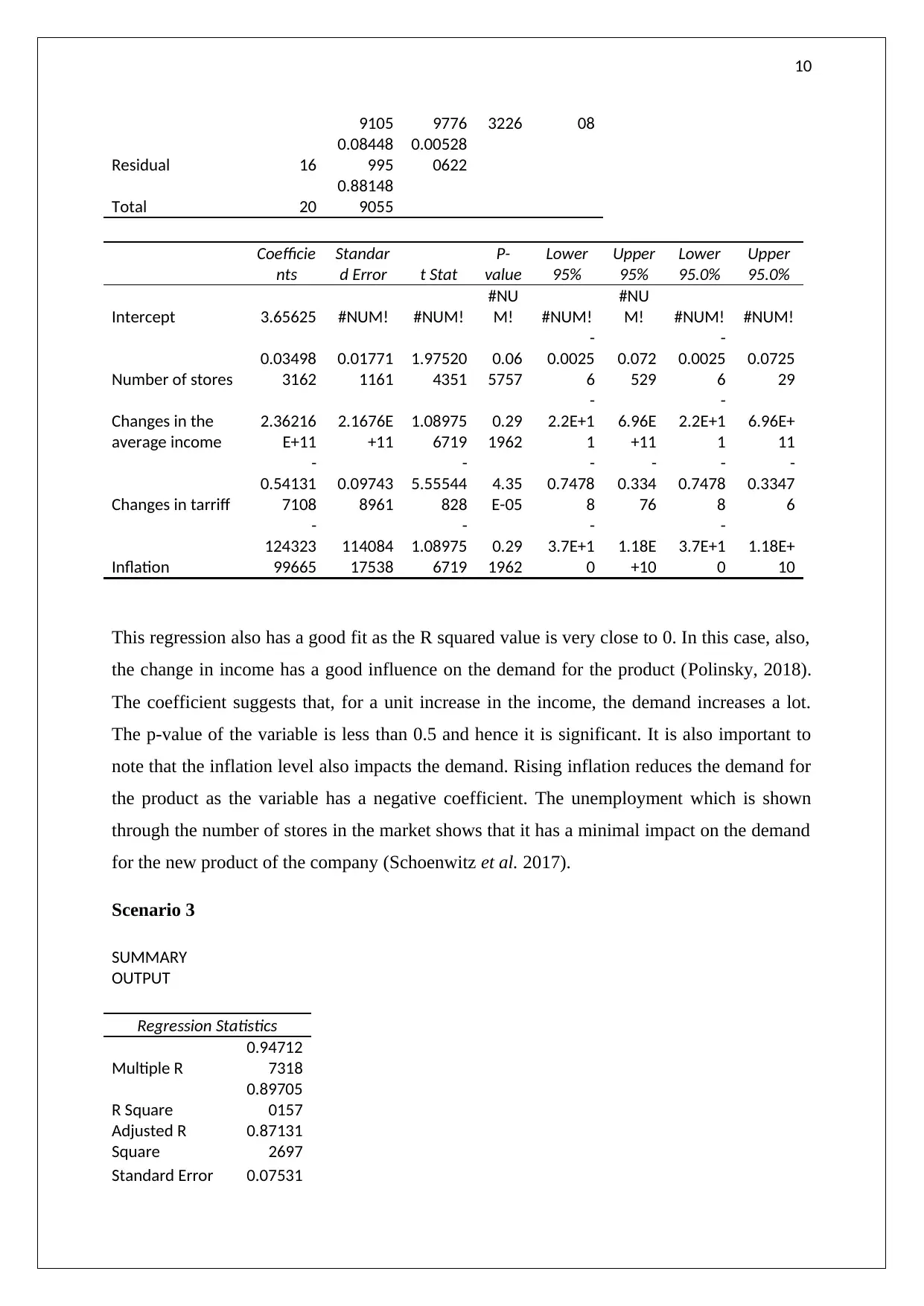
This regression also has a good fit as the R squared value is very close to 0. In this case, also,
the change in income has a good influence on the demand for the product (Polinsky, 2018).
The coefficient suggests that, for a unit increase in the income, the demand increases a lot.
The p-value of the variable is less than 0.5 and hence it is significant. It is also important to
note that the inflation level also impacts the demand. Rising inflation reduces the demand for
the product as the variable has a negative coefficient. The unemployment which is shown
through the number of stores in the market shows that it has a minimal impact on the demand
for the new product of the company (Schoenwitz et al. 2017).
Scenario 3
SUMMARY
OUTPUT
Regression Statistics
Multiple R
0.94712
7318
R Square
0.89705
0157
Adjusted R
Square
0.87131
2697
Standard Error 0.07531
9105 9776 3226 08
Residual 16
0.08448
995
0.00528
0622
Total 20
0.88148
9055
Coefficie
nts
Standar
d Error t Stat
P-
value
Lower
95%
Upper
95%
Lower
95.0%
Upper
95.0%
Intercept 3.65625 #NUM! #NUM!
#NU
M! #NUM!
#NU
M! #NUM! #NUM!
Number of stores
0.03498
3162
0.01771
1161
1.97520
4351
0.06
5757
-
0.0025
6
0.072
529
-
0.0025
6
0.0725
29
Changes in the
average income
2.36216
E+11
2.1676E
+11
1.08975
6719
0.29
1962
-
2.2E+1
1
6.96E
+11
-
2.2E+1
1
6.96E+
11
Changes in tarriff
-
0.54131
7108
0.09743
8961
-
5.55544
828
4.35
E-05
-
0.7478
8
-
0.334
76
-
0.7478
8
-
0.3347
6
Inflation
-
124323
99665
114084
17538
-
1.08975
6719
0.29
1962
-
3.7E+1
0
1.18E
+10
-
3.7E+1
0
1.18E+
10
This regression also has a good fit as the R squared value is very close to 0. In this case, also,
the change in income has a good influence on the demand for the product (Polinsky, 2018).
The coefficient suggests that, for a unit increase in the income, the demand increases a lot.
The p-value of the variable is less than 0.5 and hence it is significant. It is also important to
note that the inflation level also impacts the demand. Rising inflation reduces the demand for
the product as the variable has a negative coefficient. The unemployment which is shown
through the number of stores in the market shows that it has a minimal impact on the demand
for the new product of the company (Schoenwitz et al. 2017).
Scenario 3
SUMMARY
OUTPUT
Regression Statistics
Multiple R
0.94712
7318
R Square
0.89705
0157
Adjusted R
Square
0.87131
2697
Standard Error 0.07531
Paraphrase This Document
Need a fresh take? Get an instant paraphrase of this document with our AI Paraphraser
11
1503
Observations 21
ANOVA
df SS MS F
Signific
ance F
Regression 4
0.79073
9895
0.19768
4974
34.85
387
1.03E-
07
Residual 16
0.09074
916
0.00567
1822
Total 20
0.88148
9055
Coefficie
nts
Standar
d Error t Stat
P-
value
Lower
95%
Upper
95%
Lower
95.0%
Upper
95.0%
Intercept
3.65820
3125
3712577
.415
9.85354
E-07
0.999
999
-
787030
9
78703
16
-
787030
9
787031
6
Number of
stores
0.03666
3217
0.01836
1564
1.99673
7187
0.063
158
-
0.00226
0.075
588
-
0.0022
6
0.0755
88
Change in
average income
-
1803785
8586
3.93852
E+11
-
0.04579
856
0.964
038
-
8.5E+11
8.17E
+11
-
8.5E+1
1
8.17E+
11
Change in tariff
-
1.10780
9849
0.20174
5426
-
5.49112
7452
4.93E
-05
-
1.53549
-
0.680
13
-
1.5354
9
-
0.6801
3
Inflation
5521793
44.5
1205669
6583
0.04579
856
0.964
038
-
2.5E+10
2.61E
+10
-
2.5E+1
0
2.61E+
10
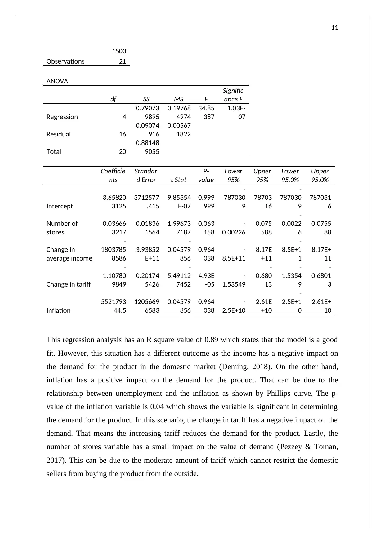
This regression analysis has an R square value of 0.89 which states that the model is a good
fit. However, this situation has a different outcome as the income has a negative impact on
the demand for the product in the domestic market (Deming, 2018). On the other hand,
inflation has a positive impact on the demand for the product. That can be due to the
relationship between unemployment and the inflation as shown by Phillips curve. The p-
value of the inflation variable is 0.04 which shows the variable is significant in determining
the demand for the product. In this scenario, the change in tariff has a negative impact on the
demand. That means the increasing tariff reduces the demand for the product. Lastly, the
number of stores variable has a small impact on the value of demand (Pezzey & Toman,
2017). This can be due to the moderate amount of tariff which cannot restrict the domestic
sellers from buying the product from the outside.
1503
Observations 21
ANOVA
df SS MS F
Signific
ance F
Regression 4
0.79073
9895
0.19768
4974
34.85
387
1.03E-
07
Residual 16
0.09074
916
0.00567
1822
Total 20
0.88148
9055
Coefficie
nts
Standar
d Error t Stat
P-
value
Lower
95%
Upper
95%
Lower
95.0%
Upper
95.0%
Intercept
3.65820
3125
3712577
.415
9.85354
E-07
0.999
999
-
787030
9
78703
16
-
787030
9
787031
6
Number of
stores
0.03666
3217
0.01836
1564
1.99673
7187
0.063
158
-
0.00226
0.075
588
-
0.0022
6
0.0755
88
Change in
average income
-
1803785
8586
3.93852
E+11
-
0.04579
856
0.964
038
-
8.5E+11
8.17E
+11
-
8.5E+1
1
8.17E+
11
Change in tariff
-
1.10780
9849
0.20174
5426
-
5.49112
7452
4.93E
-05
-
1.53549
-
0.680
13
-
1.5354
9
-
0.6801
3
Inflation
5521793
44.5
1205669
6583
0.04579
856
0.964
038
-
2.5E+10
2.61E
+10
-
2.5E+1
0
2.61E+
10
This regression analysis has an R square value of 0.89 which states that the model is a good
fit. However, this situation has a different outcome as the income has a negative impact on
the demand for the product in the domestic market (Deming, 2018). On the other hand,
inflation has a positive impact on the demand for the product. That can be due to the
relationship between unemployment and the inflation as shown by Phillips curve. The p-
value of the inflation variable is 0.04 which shows the variable is significant in determining
the demand for the product. In this scenario, the change in tariff has a negative impact on the
demand. That means the increasing tariff reduces the demand for the product. Lastly, the
number of stores variable has a small impact on the value of demand (Pezzey & Toman,
2017). This can be due to the moderate amount of tariff which cannot restrict the domestic
sellers from buying the product from the outside.
12
Scenario 4
SUMMARY
OUTPUT
Regression Statistics
Multiple R
0.8378
13612
R Square
0.7019
31649
Adjusted R
Square
0.5905
07822
Standard Error
0.1243
20267
Observations 21
ANOVA
df SS MS F
Signific
ance F
Regression 4
0.61874
5066
0.15468
6266
13.34
463
5.72E-
05
Residual 17
0.26274
3989
0.01545
5529
Total 21
0.88148
9055
Coeffici
ents
Standar
d Error t Stat
P-
value
Lower
95%
Upper
95%
Lower
95.0%
Upper
95.0%
Intercept 3.625 #NUM! #NUM!
#NU
M! #NUM!
#NUM
! #NUM! #NUM!
Number of stores
0.0720
22271
0.02836
7823
2.53887
2013
0.021
189
0.01217
1
0.131
873
0.0121
71
0.1318
73
Change in the
average income
505065
2636
2545493
2641
0.19841
5478
0.845
073
-
4.9E+10
5.88E
+10
-
4.9E+1
0
5.88E+
10
Change in tariff 0 0 65535
#NU
M! 0 0 0 0
inflation
-
360760
9026
1818209
4744
-
0.19841
5478
0.845
073
-
4.2E+10
3.48E
+10
-
4.2E+1
0
3.48E+
10
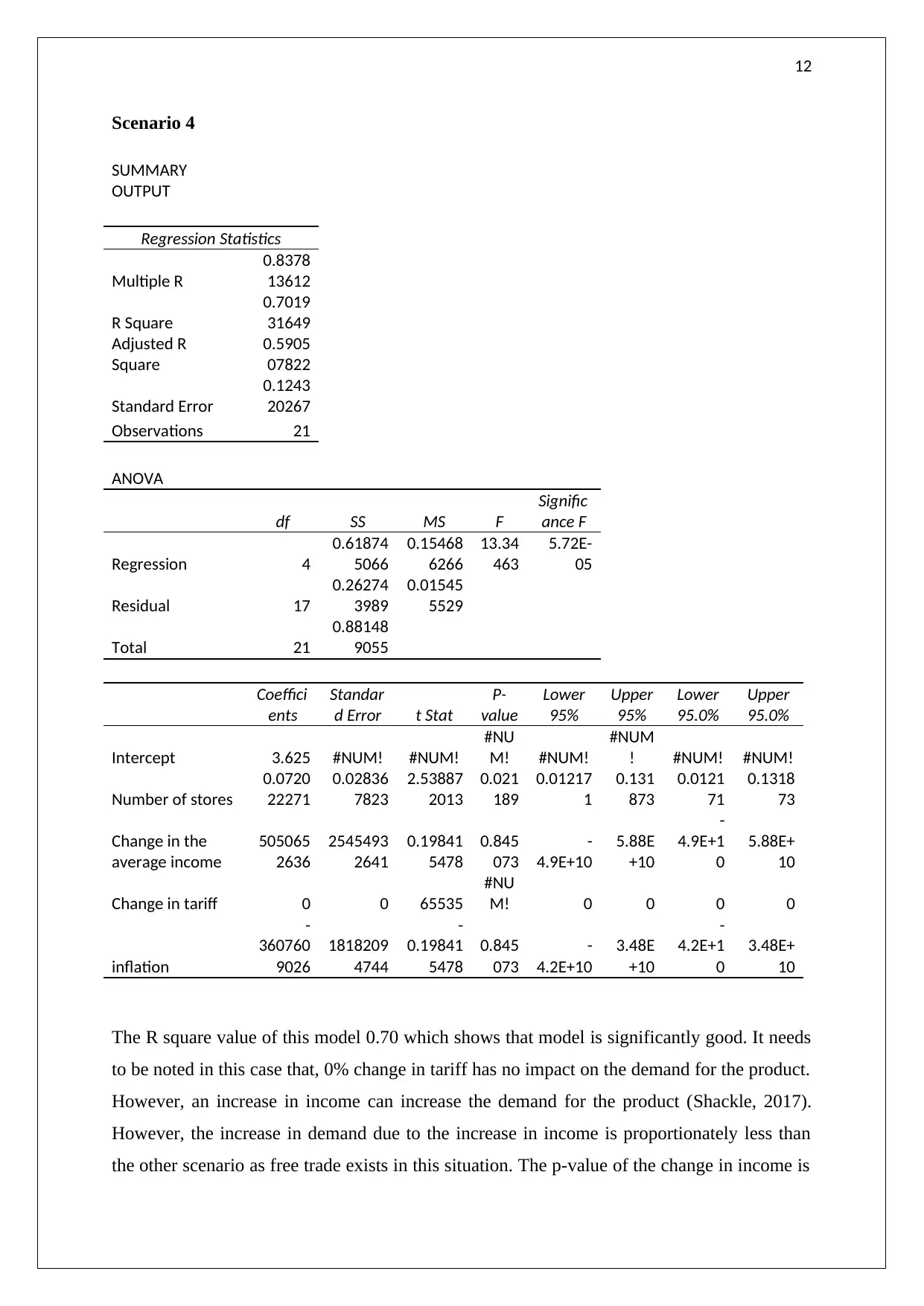
The R square value of this model 0.70 which shows that model is significantly good. It needs
to be noted in this case that, 0% change in tariff has no impact on the demand for the product.
However, an increase in income can increase the demand for the product (Shackle, 2017).
However, the increase in demand due to the increase in income is proportionately less than
the other scenario as free trade exists in this situation. The p-value of the change in income is
Scenario 4
SUMMARY
OUTPUT
Regression Statistics
Multiple R
0.8378
13612
R Square
0.7019
31649
Adjusted R
Square
0.5905
07822
Standard Error
0.1243
20267
Observations 21
ANOVA
df SS MS F
Signific
ance F
Regression 4
0.61874
5066
0.15468
6266
13.34
463
5.72E-
05
Residual 17
0.26274
3989
0.01545
5529
Total 21
0.88148
9055
Coeffici
ents
Standar
d Error t Stat
P-
value
Lower
95%
Upper
95%
Lower
95.0%
Upper
95.0%
Intercept 3.625 #NUM! #NUM!
#NU
M! #NUM!
#NUM
! #NUM! #NUM!
Number of stores
0.0720
22271
0.02836
7823
2.53887
2013
0.021
189
0.01217
1
0.131
873
0.0121
71
0.1318
73
Change in the
average income
505065
2636
2545493
2641
0.19841
5478
0.845
073
-
4.9E+10
5.88E
+10
-
4.9E+1
0
5.88E+
10
Change in tariff 0 0 65535
#NU
M! 0 0 0 0
inflation
-
360760
9026
1818209
4744
-
0.19841
5478
0.845
073
-
4.2E+10
3.48E
+10
-
4.2E+1
0
3.48E+
10
The R square value of this model 0.70 which shows that model is significantly good. It needs
to be noted in this case that, 0% change in tariff has no impact on the demand for the product.
However, an increase in income can increase the demand for the product (Shackle, 2017).
However, the increase in demand due to the increase in income is proportionately less than
the other scenario as free trade exists in this situation. The p-value of the change in income is
⊘ This is a preview!⊘
Do you want full access?
Subscribe today to unlock all pages.
Trusted by 1+ million students worldwide
1 out of 16
Related Documents


Your All-in-One AI-Powered Toolkit for Academic Success.
+13062052269
info@desklib.com
Available 24*7 on WhatsApp / Email
![[object Object]](/_next/static/media/star-bottom.7253800d.svg)
Unlock your academic potential
Copyright © 2020–2026 A2Z Services. All Rights Reserved. Developed and managed by ZUCOL.