ECON 940 Statistics: Analyzing Consumer Behavior in Car Market

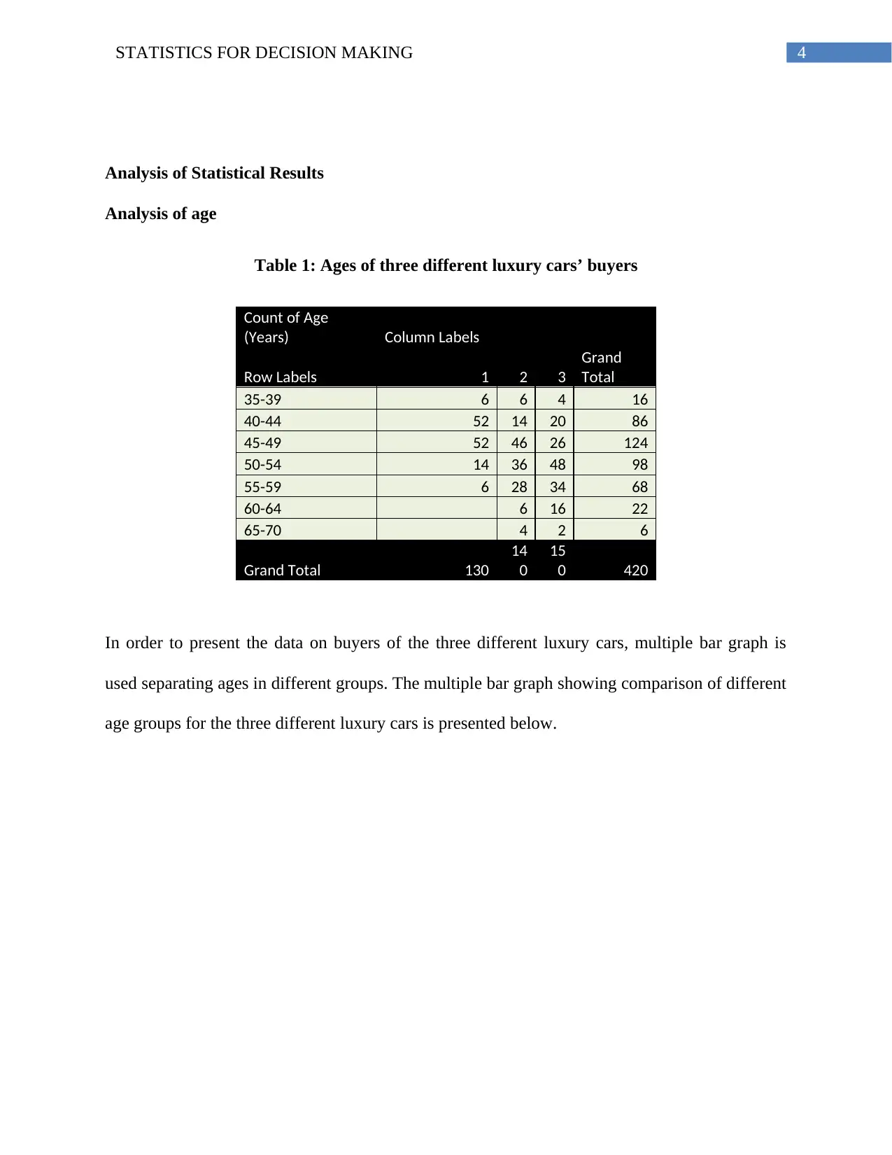
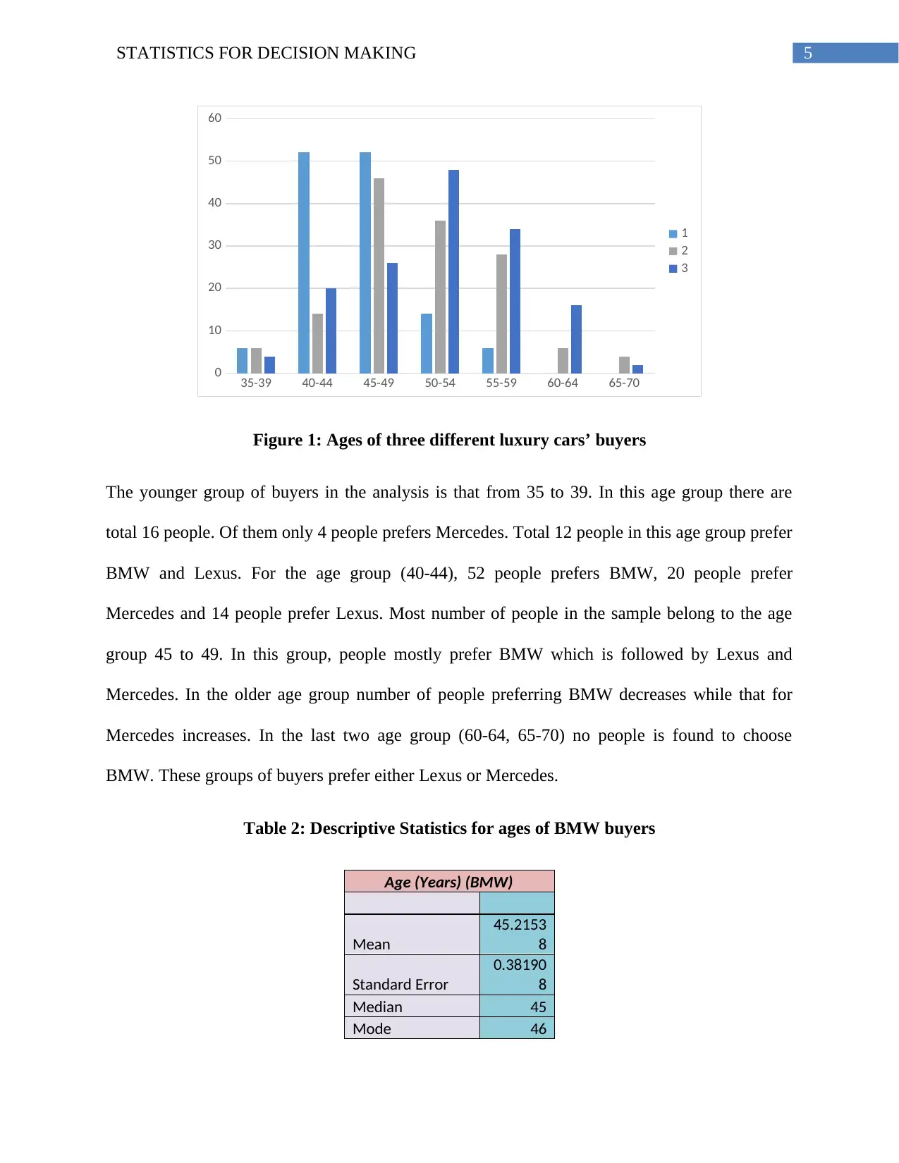
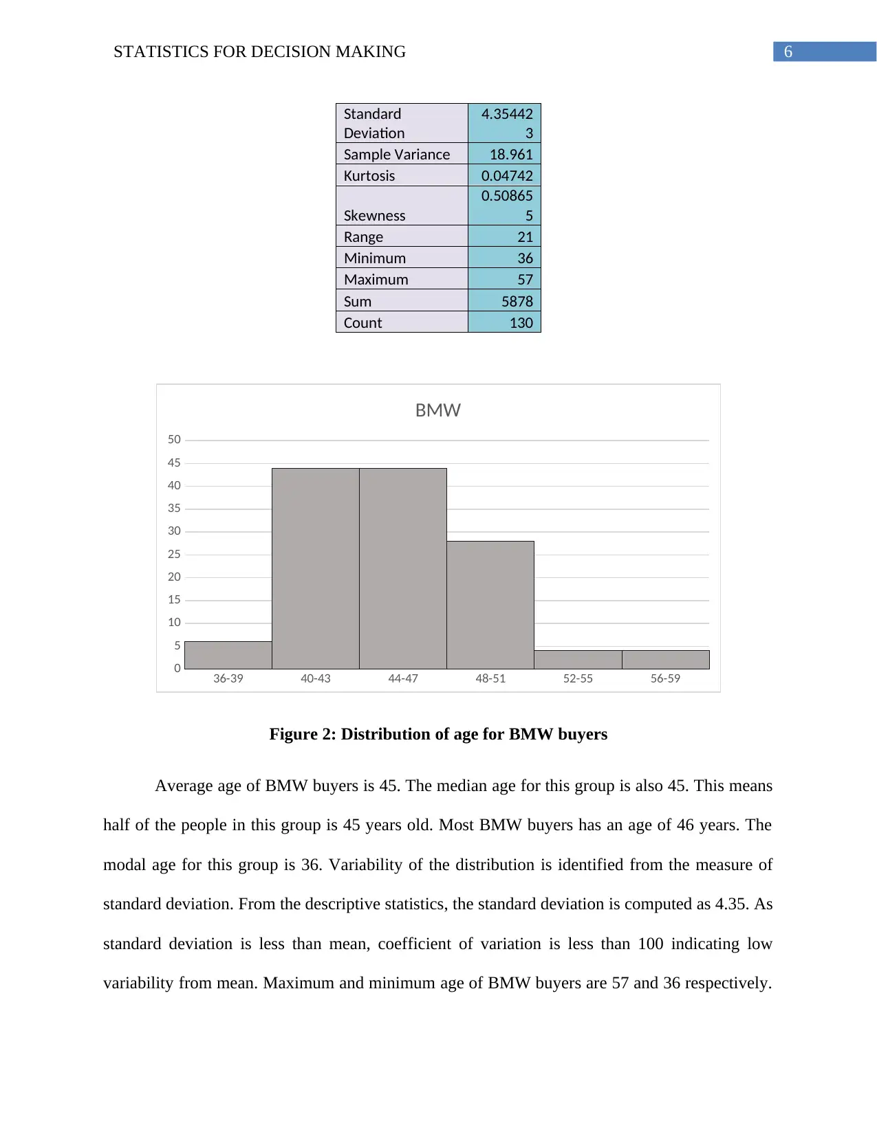
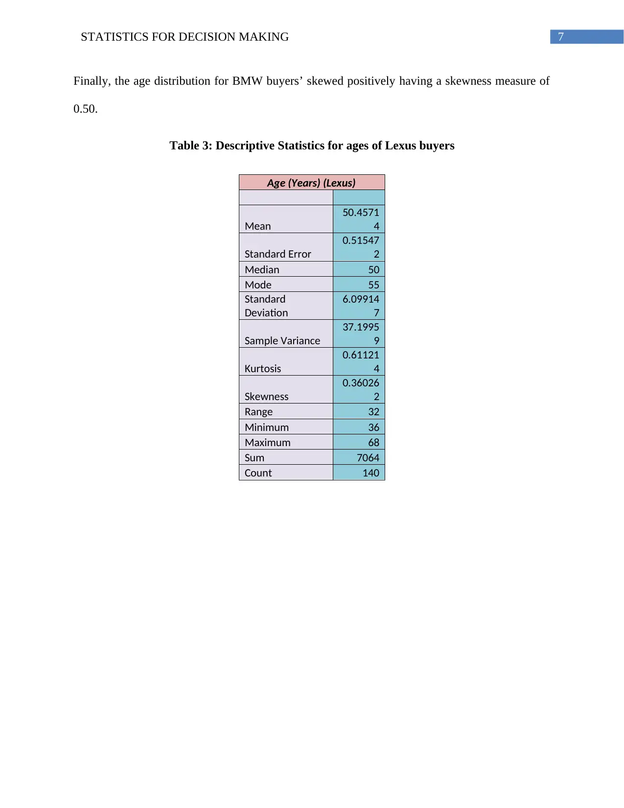
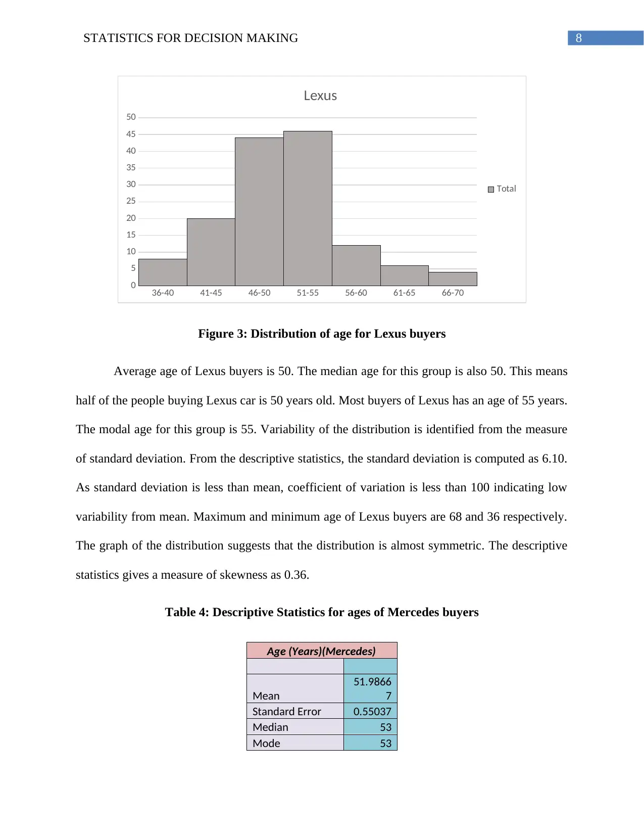
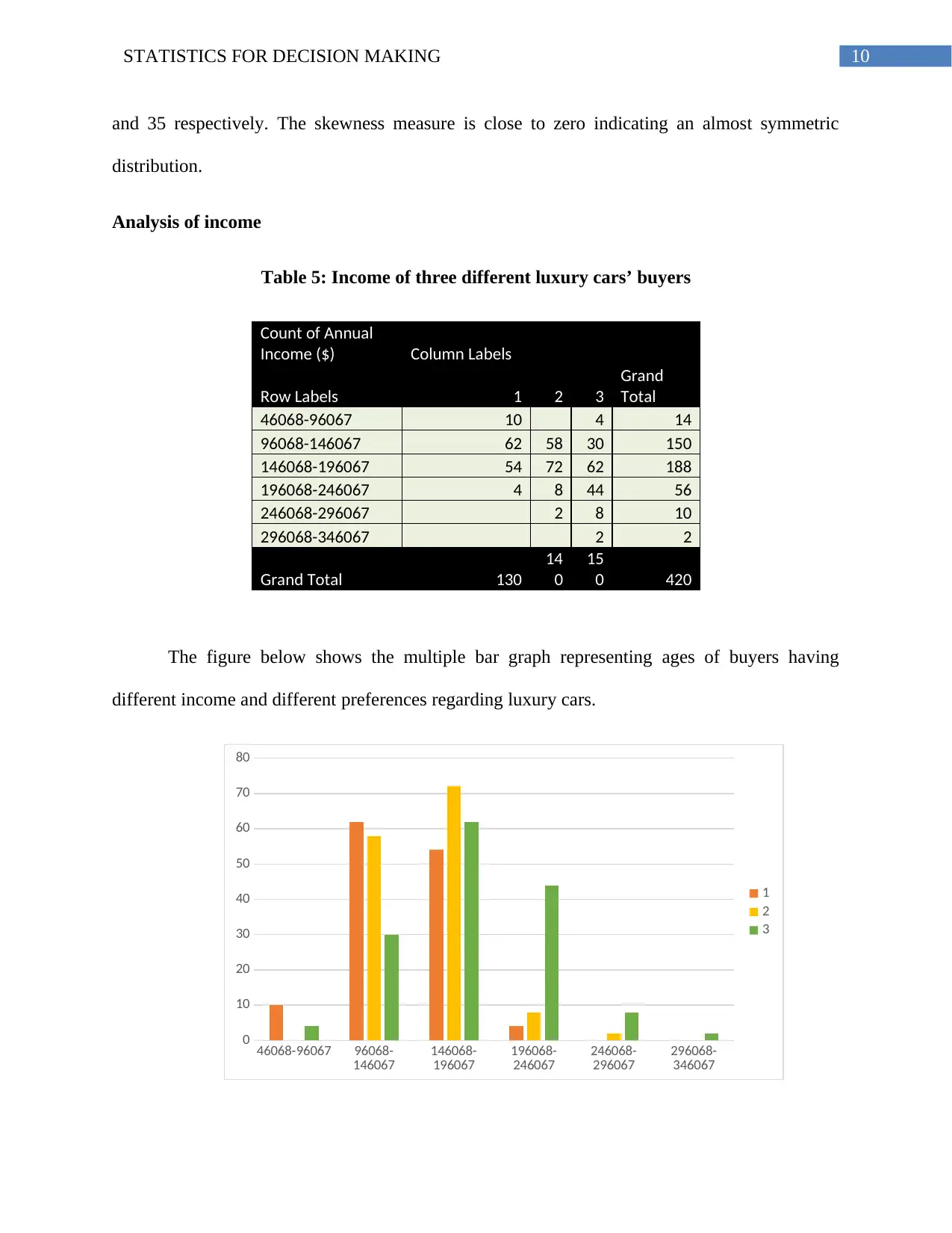
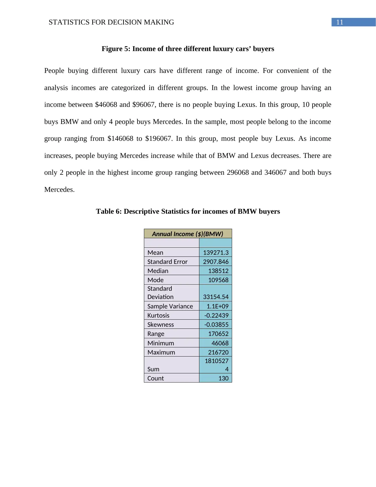
This business report analyzes the demand for BMW, Lexus, and Mercedes luxury cars based on customer age, income, and education. A survey of 420 samples reveals that Mercedes is the most preferred, followed by Lexus and BMW. BMW buyers tend to be younger with lower incomes and fewer years of education. Statistical analysis, including ANOVA tests, confirms significant differences in mean income, age, and education among the buyer groups. Logistic regression indicates that older individuals with higher incomes and more education are more likely to purchase Mercedes. The report uses descriptive statistics to understand the distribution of age, income, and education, and provides insights into consumer preferences to help car sellers target their consumers and maximize revenue.

Running Head: STATISTICS FOR DECISION MAKING
Statistics for Decision Making
Name of the Student
Name of the University
Student ID

1STATISTICS FOR DECISION MAKING
Executive Summary
Consumer behavior plays an important role in business decision. For normal goods, price is the
main influencing factor of demand. However, in case of luxury goods, there are factors above
prices that needs to be considered in estimating demand. The business report intends to analyze
the demand for three different luxury cars. The three selected luxury car models are BMW,
Lexus and Mercedes. Customer preferences are evaluated based on their age, income and
education years. 420 samples are considered to have an overall idea of buyers’ preference
towards different luxury car models. Among the total sample surveyed, most people preferred to
buy Mercedes cars. After Mercedes the most popular luxury cars is Lexus and then BMW.
Group of buyers for BMW are relatively younger. They have income less than group of buyers
for two other luxury cars and have lesser year of education. The average age, income and
education years are relatively lower as compared to buyers of Lexus and Mercedes. There exists
significant statistical differences in mean income, age and education years among the three
different buyers group of three different luxury cars. The statistical result also shows that with
people belong to older age group, higher income bracket and a higher number of education years
tends to buy Mercedes over BMW or Mercedes.

2STATISTICS FOR DECISION MAKING
Table of Contents
Introduction......................................................................................................................................3
Business Problem.........................................................................................................................3
Statistical Problem.......................................................................................................................3
Analysis of Statistical Results.........................................................................................................4
Analysis of age............................................................................................................................4
Analysis of income......................................................................................................................9
Analysis of Education................................................................................................................14
Test for the Difference in the Average Household Ages...........................................................19
Test for the Difference in the Average Income of Different Households.................................20
Test for the Difference in the Average Education of Different Households.............................22
2.7 Regression Analysis.............................................................................................................23
Conclusion and Recommendation.................................................................................................26

3STATISTICS FOR DECISION MAKING
Introduction
The Automobile Association conducts a survey to estimate demand for different group of
buyers. The knowledge regarding customer preferences help the car seller to set their targeted
consumer and maximize their revenue. The business problem has been discussed using different
statistical tools.
Business Problem
The main problem of every business is to maximize its profit. For this, business owners
should know their customer group, preferences and other information related to profiles of
customer group. To accomplish this goal for sellers of luxury cars, the association conducts the
survey. Buyers are grouped according to their age, income and education years. This report
addresses the business problem of demand determination. The detailed knowledge regarding
buyers profile helps the business to achieve its target.
Statistical Problem
Problem of the business is addressed with help of different statistical tool. The nature of
distribution age, income and education is determined from summary statistics related to the
distribution. The descriptive statistics provides information regarding shape, location and
variability of the relevant distribution. To test independency of average age, average income and
average education year’s three different ANOVA tests are performed. Lastly, to find out whether
buyers with a higher age, income and more education years tend to buy Mercedes to Lexus and
BMW logistic regression has been done.

4STATISTICS FOR DECISION MAKING
Analysis of Statistical Results
Analysis of age
Table 1: Ages of three different luxury cars’ buyers
Count of Age
(Years) Column Labels
Row Labels 1 2 3
Grand
Total
35-39 6 6 4 16
40-44 52 14 20 86
45-49 52 46 26 124
50-54 14 36 48 98
55-59 6 28 34 68
60-64 6 16 22
65-70 4 2 6
Grand Total 130
14
0
15
0 420
In order to present the data on buyers of the three different luxury cars, multiple bar graph is
used separating ages in different groups. The multiple bar graph showing comparison of different
age groups for the three different luxury cars is presented below.

5STATISTICS FOR DECISION MAKING
35-39 40-44 45-49 50-54 55-59 60-64 65-70
0
10
20
30
40
50
60
1
2
3
Figure 1: Ages of three different luxury cars’ buyers
The younger group of buyers in the analysis is that from 35 to 39. In this age group there are
total 16 people. Of them only 4 people prefers Mercedes. Total 12 people in this age group prefer
BMW and Lexus. For the age group (40-44), 52 people prefers BMW, 20 people prefer
Mercedes and 14 people prefer Lexus. Most number of people in the sample belong to the age
group 45 to 49. In this group, people mostly prefer BMW which is followed by Lexus and
Mercedes. In the older age group number of people preferring BMW decreases while that for
Mercedes increases. In the last two age group (60-64, 65-70) no people is found to choose
BMW. These groups of buyers prefer either Lexus or Mercedes.
Table 2: Descriptive Statistics for ages of BMW buyers
Age (Years) (BMW)
Mean
45.2153
8
Standard Error
0.38190
8
Median 45
Mode 46

6STATISTICS FOR DECISION MAKING
Standard
Deviation
4.35442
3
Sample Variance 18.961
Kurtosis 0.04742
Skewness
0.50865
5
Range 21
Minimum 36
Maximum 57
Sum 5878
Count 130
36-39 40-43 44-47 48-51 52-55 56-59
0
5
10
15
20
25
30
35
40
45
50
BMW
Figure 2: Distribution of age for BMW buyers
Average age of BMW buyers is 45. The median age for this group is also 45. This means
half of the people in this group is 45 years old. Most BMW buyers has an age of 46 years. The
modal age for this group is 36. Variability of the distribution is identified from the measure of
standard deviation. From the descriptive statistics, the standard deviation is computed as 4.35. As
standard deviation is less than mean, coefficient of variation is less than 100 indicating low
variability from mean. Maximum and minimum age of BMW buyers are 57 and 36 respectively.

7STATISTICS FOR DECISION MAKING
Finally, the age distribution for BMW buyers’ skewed positively having a skewness measure of
0.50.
Table 3: Descriptive Statistics for ages of Lexus buyers
Age (Years) (Lexus)
Mean
50.4571
4
Standard Error
0.51547
2
Median 50
Mode 55
Standard
Deviation
6.09914
7
Sample Variance
37.1995
9
Kurtosis
0.61121
4
Skewness
0.36026
2
Range 32
Minimum 36
Maximum 68
Sum 7064
Count 140

8STATISTICS FOR DECISION MAKING
36-40 41-45 46-50 51-55 56-60 61-65 66-70
0
5
10
15
20
25
30
35
40
45
50
Lexus
Total
Figure 3: Distribution of age for Lexus buyers
Average age of Lexus buyers is 50. The median age for this group is also 50. This means
half of the people buying Lexus car is 50 years old. Most buyers of Lexus has an age of 55 years.
The modal age for this group is 55. Variability of the distribution is identified from the measure
of standard deviation. From the descriptive statistics, the standard deviation is computed as 6.10.
As standard deviation is less than mean, coefficient of variation is less than 100 indicating low
variability from mean. Maximum and minimum age of Lexus buyers are 68 and 36 respectively.
The graph of the distribution suggests that the distribution is almost symmetric. The descriptive
statistics gives a measure of skewness as 0.36.
Table 4: Descriptive Statistics for ages of Mercedes buyers
Age (Years)(Mercedes)
Mean
51.9866
7
Standard Error 0.55037
Median 53
Mode 53

9STATISTICS FOR DECISION MAKING
Standard
Deviation
6.74062
8
Sample Variance
45.4360
6
Kurtosis -0.0195
Skewness -0.02894
Range 35
Minimum 35
Maximum 70
Sum 7798
Count 150
35-39 40-44 45-49 50-54 55-59 60-64 65-70
0
10
20
30
40
50
60
Mercedes
Total
Figure 4: Distribution of age for Mercedes buyers
Mean age of Mercedes buyers is 52. The median age for this group is also 53. This means
half of the people in this group is 53 years old. Most Mercedes buyers has an age of 53 years.
The modal age for this group is 53. From the descriptive statistics, the standard deviation is
computed as 6.74. As standard deviation is less than mean, coefficient of variation is less than
100 indicating low variability from mean. Maximum and minimum age of BMW buyers are 70

10STATISTICS FOR DECISION MAKING
and 35 respectively. The skewness measure is close to zero indicating an almost symmetric
distribution.
Analysis of income
Table 5: Income of three different luxury cars’ buyers
Count of Annual
Income ($) Column Labels
Row Labels 1 2 3
Grand
Total
46068-96067 10 4 14
96068-146067 62 58 30 150
146068-196067 54 72 62 188
196068-246067 4 8 44 56
246068-296067 2 8 10
296068-346067 2 2
Grand Total 130
14
0
15
0 420
The figure below shows the multiple bar graph representing ages of buyers having
different income and different preferences regarding luxury cars.
46068-96067 96068-
146067 146068-
196067 196068-
246067 246068-
296067 296068-
346067
0
10
20
30
40
50
60
70
80
1
2
3

11STATISTICS FOR DECISION MAKING
Figure 5: Income of three different luxury cars’ buyers
People buying different luxury cars have different range of income. For convenient of the
analysis incomes are categorized in different groups. In the lowest income group having an
income between $46068 and $96067, there is no people buying Lexus. In this group, 10 people
buys BMW and only 4 people buys Mercedes. In the sample, most people belong to the income
group ranging from $146068 to $196067. In this group, most people buy Lexus. As income
increases, people buying Mercedes increase while that of BMW and Lexus decreases. There are
only 2 people in the highest income group ranging between 296068 and 346067 and both buys
Mercedes.
Table 6: Descriptive Statistics for incomes of BMW buyers
Annual Income ($)(BMW)
Mean 139271.3
Standard Error 2907.846
Median 138512
Mode 109568
Standard
Deviation 33154.54
Sample Variance 1.1E+09
Kurtosis -0.22439
Skewness -0.03855
Range 170652
Minimum 46068
Maximum 216720
Sum
1810527
4
Count 130

12STATISTICS FOR DECISION MAKING
46068-76067 76068-106067 106068-
136067 136068-
166067 166068-
196067 196068-
226067
0
5
10
15
20
25
30
35
40
45
50
BMW
Figure 6: Distribution of income for buyers of BMW
Average income of people buying BMW is 139271 dollars. This implies people buying BMW
cars on an average has an income of 139271 dollar. Median income is 138512 dollar. Most
people buying BMW have an income of 109568. This is implied from the modal value of the
income distribution. The standard deviation is estimated as 33154.54. The standard deviation
exceeds the value mean indicating the distribution has less volatility. The skewness measure is
obtained as -0.04. This means the distribution has a slight negative skewness.

13STATISTICS FOR DECISION MAKING
Table 7: Descriptive Statistics for incomes of Lexus buyers
Annual Income ($) (Lexus)
Mean 154186.9
Standard Error 2556.425
Median 154492
Mode 179617
Standard
Deviation 30248.02
Sample Variance 9.15E+08
Kurtosis 0.963641
Skewness 0.693685
Range 152065
Minimum 96069
Maximum 248134
Sum
2158616
0
Count 140
96069-126068 126069-156068 156069-186068 186069-216068 216069-246068 246069-276068
0
10
20
30
40
50
60
Lexus
Figure 7: Distribution of income for buyers of Lexus

14STATISTICS FOR DECISION MAKING
Average income of people buying BMW is 154187 dollars. This implies people buying BMW
cars on an average has an income of 154187 dollar. Median income is 1544492 dollar. Most
people buying BMW have an income of 179617. This is implied from the modal value of the
income distribution. The standard deviation is estimated as 30248.02. The standard deviation
exceeds the value mean indicating the distribution has less volatility. The skewness measure is
obtained as 0.69. This means the distribution skewed positively.
Table 8: Descriptive Statistics for incomes of Mercedes buyers
Annual Income ($)
(Mercedes)
Mean 184423.9
Standard Error 3845.333
Median 186070
Mode 161590
Standard
Deviation 47095.52
Sample Variance 2.22E+09
Kurtosis 0.987178
Skewness 0.273966
Range 284882
Minimum 49941
Maximum 334823
Sum
2766359
2
Count 150

15STATISTICS FOR DECISION MAKING
49941-109940 109941-169940 169941-229940 229941-289940 289941-349940
0
20
40
60
80
100
120
140
Mercedes
Figure 8: Distribution of income for buyers of Mercedes
People buying Mercedes cars on an average has an income of 184423 dollars. Median income is
186070 dollar. The median income indicates that half of the people in this group has an income
of 186070. The modal income for this group is 161590.The standard deviation is estimated as
47095.2. The standard deviation exceeds the value mean indicating the distribution has less
volatility. The skewness measure is obtained as 0.27. This means the distribution skewed
positively. The skewness measure implies that income distribution of Mercedes buyers is
positively skewed.
Analysis of Education
Table 9: Education of three different luxury cars’ buyers
Count of Education
(Years) Column Labels
Row Labels 1 2 3
Grand
Total
11-13 12 34 2 48
14-16 66 52 38 156
17-19 52 44 94 190

16STATISTICS FOR DECISION MAKING
20-22 10 16 26
Grand Total 130
14
0
15
0 420
11-13 14-16 17-19 20-22
0
10
20
30
40
50
60
70
80
90
100
1
2
3
Figure 9: Education of three different luxury cars’ buyers
Buyers are divided into four group based on their years of education. In the lowest education
years (11-13), 34 people buy Lexus, 12 people buy BMW and only 2 people buy Mercedes. In
the education group of 14 – 16 years, most people buy BMW. Buyers having education years of
17-19, prefer to buy Mercedes. For the education group of 20-22, there are no buyers buying
BMW. In this group, people buy either Lexus or Mercedes.
Table 10: Descriptive Statistics for education years of BMW buyers
Education (Years) (BMW)
Mean
15.8307
7
Standard Error
0.16092
3
Median 16

17STATISTICS FOR DECISION MAKING
Mode 16
Standard
Deviation
1.83479
9
Sample Variance
3.36648
8
Kurtosis -0.17288
Skewness -0.4345
Range 8
Minimum 11
Maximum 19
Sum 2058
Count 130
11 13 14 15 16 17 18 19
0.00%
5.00%
10.00%
15.00%
20.00%
25.00%
BMW
Figure 10: Distribution of education years for buyers of BMW
The average education year for BMW buyers is 16. The median and modal education year is
almost same as mean education years. In this group, buyers have a maximum education years of
19 and minimum education years of 11. The descriptive statistics gives standard deviation
measure as 1.83. The smaller value of standard deviation implies that the distribution is less
volatile. The distribution is almost symmetric as implied from an equal value of mean, median
and mode.

18STATISTICS FOR DECISION MAKING

19STATISTICS FOR DECISION MAKING
Table 11: Descriptive Statistics for education years of Lexus buyers
Education (Years) (Lexus)
Mean 15.8
Standard Error
0.20406959
3
Median 16
Mode 16
Standard
Deviation
2.41458398
6
Sample Variance
5.83021582
7
Kurtosis
-
0.97728269
8
Skewness
0.16971991
8
Range 9
Minimum 12
Maximum 21
Sum 2212
Count 140
12 13 14 15 16 17 18 19 20 21
0.00%
2.00%
4.00%
6.00%
8.00%
10.00%
12.00%
14.00%
16.00%
18.00%
Lexus
Figure 11: Distribution of education years for buyers of Lexus

20STATISTICS FOR DECISION MAKING
The average education year for Lexus buyers is same as that of BMW buyers. The mean
education year is 16. The median and modal education year is almost same as mean education
years. In this group, buyers have a maximum education years of 21 and minimum education
years of 12. The descriptive statistics gives standard deviation measure as 2.41. The smaller
value of standard deviation implies that the distribution is less volatile. The distribution is almost
symmetric as implied from an equal value of mean, median and mode.
Table 12: Descriptive Statistics for education years of Mercedes buyers
Education (Years) (Mercedes)
Mean
17.2933
3
Standard Error
0.14206
7
Median 17
Mode 17
Standard Deviation
1.73996
3
Sample Variance
3.02747
2
Kurtosis
0.03963
3
Skewness
0.08167
6
Range 9
Minimum 13
Maximum 22
Sum 2594
Count 150

21STATISTICS FOR DECISION MAKING
13 14 15 16 17 18 19 20 21 22
0.00%
5.00%
10.00%
15.00%
20.00%
25.00%
30.00%
35.00%
40.00%
Mercedes
Figure 12: Distribution of education years for buyers of Mercedes
The average education year for Mercedes buyers is 17. The median and modal education year is
almost same as mean education years. In this group, buyers have a maximum education years of
22 and minimum education years of 13. The descriptive statistics gives standard deviation
measure as 3.02. The estimated standard deviation is less than the estimated average implying
less variability of the distribution. The distribution of education years for buyers of Mercedes are
almost symmetric. This is indicated from the equal value of mean, median and mode.
Test for the Difference in the Average Household Ages
Here, testing is to be done for the differences in the average age of the buyers with
respect to different types of luxury cars. To conduct this test, the most appropriate technique that
can be used is the Analysis of Variance (ANOVA) technique.
Let M1 be average age of the household owning BMW cars, M2 be the average age of the
household owning Lexus cars and M3 be the average age of the household owning Mercedes

22STATISTICS FOR DECISION MAKING
cars. Thus, in order to test the difference in the average ages, the following null and alternate
hypothesis can be framed:
Null Hypothesis (H01): M1 = M2 = M3
Alternate Hypothesis (HA1): M1 ≠ M2 ≠ M3
The null hypothesis is rejected at 95 percent confidence interval if the observed value of
the F-statistic is greater than the tabulated (Critical) value of the F-statistic. From the results
obtained from the ANOVA test, it can be seen that the observed value of the F-statistic is 49.8
which is quite higher than the tabulated (critical) value of the F-statistic (3.017) for 419 degrees
of freedom. Thus, it can be said that the null hypothesis (H01) for the test is rejected. Thus, it can
be said that the average household ages of the households owning different types of cars such as
BMW, Lexus and Mercedes are significantly different from each other.
Table 13: Results of ANOVA for testing difference in the average household ages
SUMMARY
Groups Count Sum Average Variance
1 130 5878 45.21538 18.961
2 140 7064 50.45714 37.19959
3 150 7798 51.98667 45.43606
ANOVA
Source of Variation SS df MS F P-value F crit
Between Groups
3436.36
2 2
1718.18
1
49.8017
1 4.02787E-20
3.01735
7
Within Groups
14386.6
9
41
7
34.5004
4
Total
17823.0
5
41
9

23STATISTICS FOR DECISION MAKING
Test for the Difference in the Average Income of Different Households
Here, testing is to be done for the differences in the average income of the buyers
belonging to the households buying different types of luxury cars. To conduct this test, the most
appropriate technique that can be used is the Analysis of Variance (ANOVA) technique.
Let I1 be average income of the household owning BMW cars, I2 be the average age of
the household owning Lexus cars and I3 be the average age of the household owning Mercedes
cars. Thus, in order to test the difference in the average ages, the following null and alternate
hypothesis can be framed:
Null Hypothesis (H02): I1 = I 2 = I 3
Alternate Hypothesis (HA2): I 1 ≠ I 2 ≠ I 3
The null hypothesis is rejected at 95 percent confidence interval if the observed value of
the F-statistic is greater than the tabulated (Critical) value of the F-statistic. From the results
obtained from the ANOVA test, it can be seen that the observed value of the F-statistic is
52.1761 which is quite higher than the tabulated (critical) value of the F-statistic (3.017) for 419
degrees of freedom. Thus, the null hypothesis (H02) for the test is rejected. Thus, it can be said
that the average income of the households owning different types of cars such as BMW, Lexus
and Mercedes are significantly different from each other.
Table 14: Results of ANOVA for testing difference in the average household incomes
SUMMARY
Groups Count Sum Average Variance
1 130 18105274 139271.3 1.1E+09
2 140 21586160 154186.9 9.15E+08
3 150 27663592 184423.9 2.22E+09

24STATISTICS FOR DECISION MAKING

25STATISTICS FOR DECISION MAKING
ANOVA
Source of Variation SS df MS F P-value F crit
Between Groups 1.5E+11 2 7.5E+10
52.176
1
5.98E-
21 3.017357
Within Groups 5.99E+11
41
7 1.44E+09
Total 7.49E+11
41
9
Test for the Difference in the Average Education of Different Households
Here, testing is to be done for the differences in the average years of education of the
buyers belonging to the households owning different types of luxury cars. To conduct this test,
the most appropriate technique that can be used is the Analysis of Variance (ANOVA)
technique.
Let E1 be average years of education of the household owning BMW cars, E2 be the
average years of education of the household owning Lexus cars and E3 be the average years of
education of the household owning Mercedes cars. Thus, in order to test the difference in the
average number of years of education, the following null and alternate hypothesis can be framed:
Null Hypothesis (H03): E 1 = E 2 = E 3
Alternate Hypothesis (HA3): E 1 ≠ E 2 ≠ E 3
The null hypothesis is rejected at 95 percent confidence interval if the observed value of
the F-statistic is greater than the tabulated (Critical) value of the F-statistic. From the results
obtained from the ANOVA test, it can be seen that the observed value of the F-statistic is
25.9257 which is quite higher than the tabulated (critical) value of the F-statistic (3.017) for 419
degrees of freedom. Thus, the null hypothesis (H03) for the test is rejected. Thus, it can be said

26STATISTICS FOR DECISION MAKING
that the average number of years of education of the households owning different types of cars
such as BMW, Lexus and Mercedes are significantly different from each other.
Table 15: Results of ANOVA for testing difference in the average household incomes
SUMMARY
Groups Count Sum Average Variance
1 130 2058 15.83077 3.366488
2 140 2212 15.8 5.830216
3 150 2594 17.29333 3.027472
ANOVA
Source of Variation SS df MS F P-value F crit
Between Groups
210.858
3 2
105.429
2
25.9256
6 2.44085E-11
3.01735
7
Within Groups 1695.77
41
7
4.06659
5
Total
1906.62
9
41
9
2.7 Regression Analysis
There has been a claim that if the number of years of education and income is higher in
the older people, then the preference of the luxury cars such as Mercedes is higher than the
preference for BMW and Lexus. In order to test this claim, regression analysis needs to be
conducted. In this case, the preference of the cars is the dependent variable which is not
continuous, but categorical. Thus, linear regression cannot be modelled to test this claim. Binary
Logistic Regression has to be conducted here. It has been observed from the analysis that the
proportion of the sample preferring Mercedes is 0.36 and that of the people preferring Lexus or
BMW is 0.64. The table of the proportions is attached as below. In the table, 1 represents the
Mercedes cars and 0 represents BMW or Lexus cars.

27STATISTICS FOR DECISION MAKING

28STATISTICS FOR DECISION MAKING
Table 16: Proportion of People Preferring Mercedes and BMW or Lexus
Variable Categories Frequencies %
Car 0 270 64.286
1 150 35.714
The results obtained from the analysis of the model and the model details are provided in
the table attached below. The effects of income, age and number of years of education on the
preference of the cars can be easily understood from the model summary.
Table 17: Logistic Regression Coefficients
Model parameters (Variable Car)
Source Value
Standar
d error
Wald Chi-
Square Pr > Chi²
Wald Lower
bound (95%)
Wald Upper
bound (95%)
Intercept -14.857 1.677 78.523 < 0.0001 -18.143 -11.571
Age (Years) 0.098 0.020 24.641 < 0.0001 0.059 0.136
Annual
Income ($) 0.000 0.000 47.145 < 0.0001 0.000 0.000
Education
(Years) 0.326 0.064 26.170 < 0.0001 0.201 0.451
From the table of the regression summary, it can be seen that the coefficients of all the
independent variables such as age, income and education have positive coefficients in the
prediction of the preference of the car models. Thus, it can be said that all the independent
variables have positive effect in the prediction model. The p-value (Pr > Chi²) indicates the
significance of the model. It can be seen that all the p-values are less than the level of
significance (0.05). This indicates that the independent variables play a very significant role in
the prediction model. Thus, there exists significant relationship between the independent and the
dependent variables.

29STATISTICS FOR DECISION MAKING
The log ratio in the regression gives the measure of the goodness of fit for the logistic
regression model. The p value for the log ratio has been found to be less than 0.0001, which
indicates that there is an overall significance of the independent variables in the prediction model
for predicting the preference of the luxury cars.
The model of prediction is represented with the help of the following equation:
Preference of Cars= 1
1+e (− (−14.857+0.098 × Age +0.00002× Annual Income+0.326 × Education ) )
Table 18: Goodness of Fit
Goodness of fit statistics (Variable Car)
Statistic Independent Full
Observations 420 420
Sum of weights 420.000 420.000
DF 419 416
-2 Log(Likelihood) 547.476 405.453
R²(McFadden) 0.000 0.259
R²(Cox and Snell) 0.000 0.287
R²(Nagelkerke) 0.000 0.394
AIC 549.476 413.453
SBC 553.516 429.614
Iterations 0 6
Table 19: Results of the Logistic Regression Test
Test of the null hypothesis H0: Y=0.357 (Variable Car)
Statistic DF Chi-square Pr > Chi²
-2 Log(Likelihood) 3 142.023 < 0.0001
Score 3 121.512 < 0.0001
Wald 3 86.750 < 0.0001

30STATISTICS FOR DECISION MAKING
Conclusion and Recommendation
The profiles of the customers owning three different types of cars such as BMW,
Mercedes and Lexus have been analyzed in this report. The customer profiles are based on three
different attributes – Age of the customers, Annual income of the customers and years of
education perceived by the customers. The sample of the selected customers consists of 420
customers among which 130 customers have been found to be owning BMW cars, 140 have been
found to be owning Mercedes cars and 150 have been found to be owning Lexus cars. The BMW
preferring people mostly belong to the age group of 40 to 49 years, have an average annual
income in the range of $96,068 - $196,067 and have perceived education for 14 – 19 years. The
Lexus preferring people mostly belong to the age group of 45 to 59 years, have an average
annual income in the range of $96,068 - $196,067 and have perceived education for 11 – 19
years. The Mercedes preferring people mostly belong to the age group of 50 to 59 years, have an
average annual income in the range of $146,068 - $246,067 and have perceived education for 17
– 19 years. The age distribution of the BMW preferring people have been found to be positively
skewed, the income distribution is negatively skewed and education years is symmetrically
distributed. The average age of the BMW users is 45 years with an average income of $139,271
and 16 years of education on an average. The average age of the Lexus users is 50 years with an
average income of $154,186 and 16 years of education on an average. The average age of the
Mercedes users is 52 years with an average income of $184,423 and 16 years of education on an
average. There has been significant difference in the average income, average age of the
household and the average number of years of education between the different types of car users.
There is significant influence of annual income, Education years and age of the households in the

31STATISTICS FOR DECISION MAKING
demand for Mercedes cars. There is a tendency among the older people with higher income and
high education to buy Mercedes cars than BMW or Lexus.
In order to determine the marketing strategies of all the sellers of the car brand, this
information obtained from the analysis can be used. The older people with higher education and
higher income should be the target of the Mercedes sellers. The middle aged people having
annual income between $96,068 and $196,067 must be the target of the sellers of BMW and
Lexus cars.