Econometrics Homework: Analyzing School Lunch Program & Interest Rates
VerifiedAdded on 2023/06/11
|15
|2684
|375
Homework Assignment
AI Summary
This econometrics assignment solution comprises three questions. The first question analyzes the effect of the federally funded school lunch program on student performance using data from 408 high schools, employing a regression model to assess the impact of expenditures, lunch program participation, and enrollment on math scores. The second question explores the relationship between short-term interest rates, inflation, and the federal budget surplus/deficit using time series data from 1960 to 2016, including tests for serial correlation and heteroskedasticity. The third question investigates the relationship between per capita expenditure on education and per capita GDP across 34 countries in 1980, addressing potential heteroskedasticity issues and applying White's test. The assignment uses E-views for econometric analysis and hypothesis testing, providing detailed interpretations of the results. Desklib offers this solution along with a wide array of study resources, including past papers and solved assignments, for students seeking academic support.
Research on Physical Aggression
Name of Student:
Name of University:
Course ID:
Name of Student:
Name of University:
Course ID:
Paraphrase This Document
Need a fresh take? Get an instant paraphrase of this document with our AI Paraphraser
Question 1:
Suppose we wish to estimate the effect of the federally funded school
lunch program on student performance. The file
MEAP93.xlscontainsdataon408highschools inAustraliafortheyear1993.
math10: percentage of tenth grade
rsatahighschoolreceivingapassingscoreonastandardizedmathemati
csexam.
expend: expenditures per student (in dollars).
lnchprg: percentage of students who are eligible for the
federal free lunch program.
enrol: number of student enrolment which measures school size
(a) Considered regression model:
math10=β0 +β1*log(expend i)+lnchprg i) * log(enrol i)
(b) Estimate the model using E-views and write down the fitted equation
(including the sample size, t-statistic and R-squared)
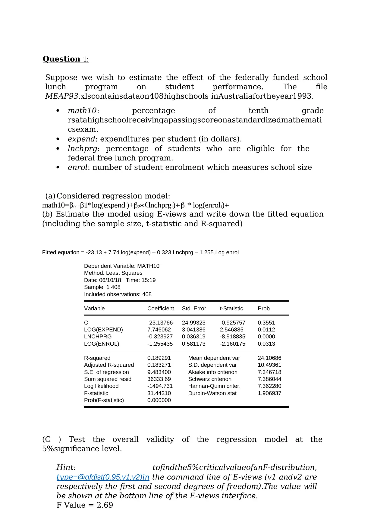
Fitted equation = -23.13 + 7.74 log(expend) – 0.323 Lnchprg – 1.255 Log enrol
Dependent Variable: MATH10
Method: Least Squares
Date: 06/10/18 Time: 15:19
Sample: 1 408
Included observations: 408
Variable Coefficient Std. Error t-Statistic Prob.
C -23.13766 24.99323 -0.925757 0.3551
LOG(EXPEND) 7.746062 3.041386 2.546885 0.0112
LNCHPRG -0.323927 0.036319 -8.918835 0.0000
LOG(ENROL) -1.255435 0.581173 -2.160175 0.0313
R-squared 0.189291 Mean dependent var 24.10686
Adjusted R-squared 0.183271 S.D. dependent var 10.49361
S.E. of regression 9.483400 Akaike info criterion 7.346718
Sum squared resid 36333.69 Schwarz criterion 7.386044
Log likelihood -1494.731 Hannan-Quinn criter. 7.362280
F-statistic 31.44310 Durbin-Watson stat 1.906937
Prob(F-statistic) 0.000000
(C ) Test the overall validity of the regression model at the
5%significance level.
Hint: tofindthe5%criticalvalueofanF-distribution,
type=@qfdist(0.95,v1,v2)in the command line of E-views (v1 andv2 are
respectively the first and second degrees of freedom).The value will
be shown at the bottom line of the E-views interface.
F Value = 2.69
Suppose we wish to estimate the effect of the federally funded school
lunch program on student performance. The file
MEAP93.xlscontainsdataon408highschools inAustraliafortheyear1993.
math10: percentage of tenth grade
rsatahighschoolreceivingapassingscoreonastandardizedmathemati
csexam.
expend: expenditures per student (in dollars).
lnchprg: percentage of students who are eligible for the
federal free lunch program.
enrol: number of student enrolment which measures school size
(a) Considered regression model:
math10=β0 +β1*log(expend i)+lnchprg i) * log(enrol i)
(b) Estimate the model using E-views and write down the fitted equation
(including the sample size, t-statistic and R-squared)
Fitted equation = -23.13 + 7.74 log(expend) – 0.323 Lnchprg – 1.255 Log enrol
Dependent Variable: MATH10
Method: Least Squares
Date: 06/10/18 Time: 15:19
Sample: 1 408
Included observations: 408
Variable Coefficient Std. Error t-Statistic Prob.
C -23.13766 24.99323 -0.925757 0.3551
LOG(EXPEND) 7.746062 3.041386 2.546885 0.0112
LNCHPRG -0.323927 0.036319 -8.918835 0.0000
LOG(ENROL) -1.255435 0.581173 -2.160175 0.0313
R-squared 0.189291 Mean dependent var 24.10686
Adjusted R-squared 0.183271 S.D. dependent var 10.49361
S.E. of regression 9.483400 Akaike info criterion 7.346718
Sum squared resid 36333.69 Schwarz criterion 7.386044
Log likelihood -1494.731 Hannan-Quinn criter. 7.362280
F-statistic 31.44310 Durbin-Watson stat 1.906937
Prob(F-statistic) 0.000000
(C ) Test the overall validity of the regression model at the
5%significance level.
Hint: tofindthe5%criticalvalueofanF-distribution,
type=@qfdist(0.95,v1,v2)in the command line of E-views (v1 andv2 are
respectively the first and second degrees of freedom).The value will
be shown at the bottom line of the E-views interface.
F Value = 2.69
H0 = The fit of intercept only model and the current model is same.
That is additional variables do not provide value taken together
H1 = The fit of intercept only model is significantly less compared
to our current model that is additional variables do make the model
significantly better.
F value is less than F statistic which means that we reject the null
hypothesis at 5% critical value. The additional variables make the
model significantly better.
(d) Does the lunch program increase student performance? Test the
hypothesis at the5%level.
H0 = The lunch model does not affect the student performance
H1 = The lunch model increases student performance
T statistic = -8.91
T value > 1
T statistic is lower than t value at 5% critical value, we therefore do
not reject the null hypothesis. The lunch program does not affect
student performance.
(e) Based on the regression output, if expend increase by 10% what is the
estimated percentage point change inmath10, holding lnchprg and enroll
constant.
math10 will change by 0.1expend units
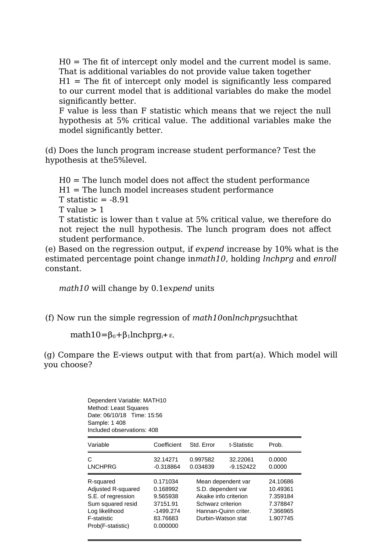
(f) Now run the simple regression of math10onlnchprgsuchthat
math10=β 0+β 1lnchprg i
(g) Compare the E-views output with that from part(a). Which model will
you choose?
Dependent Variable: MATH10
Method: Least Squares
Date: 06/10/18 Time: 15:56
Sample: 1 408
Included observations: 408
Variable Coefficient Std. Error t-Statistic Prob.
C 32.14271 0.997582 32.22061 0.0000
LNCHPRG -0.318864 0.034839 -9.152422 0.0000
R-squared 0.171034 Mean dependent var 24.10686
Adjusted R-squared 0.168992 S.D. dependent var 10.49361
S.E. of regression 9.565938 Akaike info criterion 7.359184
Sum squared resid 37151.91 Schwarz criterion 7.378847
Log likelihood -1499.274 Hannan-Quinn criter. 7.366965
F-statistic 83.76683 Durbin-Watson stat 1.907745
Prob(F-statistic) 0.000000
That is additional variables do not provide value taken together
H1 = The fit of intercept only model is significantly less compared
to our current model that is additional variables do make the model
significantly better.
F value is less than F statistic which means that we reject the null
hypothesis at 5% critical value. The additional variables make the
model significantly better.
(d) Does the lunch program increase student performance? Test the
hypothesis at the5%level.
H0 = The lunch model does not affect the student performance
H1 = The lunch model increases student performance
T statistic = -8.91
T value > 1
T statistic is lower than t value at 5% critical value, we therefore do
not reject the null hypothesis. The lunch program does not affect
student performance.
(e) Based on the regression output, if expend increase by 10% what is the
estimated percentage point change inmath10, holding lnchprg and enroll
constant.
math10 will change by 0.1expend units
(f) Now run the simple regression of math10onlnchprgsuchthat
math10=β 0+β 1lnchprg i
(g) Compare the E-views output with that from part(a). Which model will
you choose?
Dependent Variable: MATH10
Method: Least Squares
Date: 06/10/18 Time: 15:56
Sample: 1 408
Included observations: 408
Variable Coefficient Std. Error t-Statistic Prob.
C 32.14271 0.997582 32.22061 0.0000
LNCHPRG -0.318864 0.034839 -9.152422 0.0000
R-squared 0.171034 Mean dependent var 24.10686
Adjusted R-squared 0.168992 S.D. dependent var 10.49361
S.E. of regression 9.565938 Akaike info criterion 7.359184
Sum squared resid 37151.91 Schwarz criterion 7.378847
Log likelihood -1499.274 Hannan-Quinn criter. 7.366965
F-statistic 83.76683 Durbin-Watson stat 1.907745
Prob(F-statistic) 0.000000
⊘ This is a preview!⊘
Do you want full access?
Subscribe today to unlock all pages.
Trusted by 1+ million students worldwide
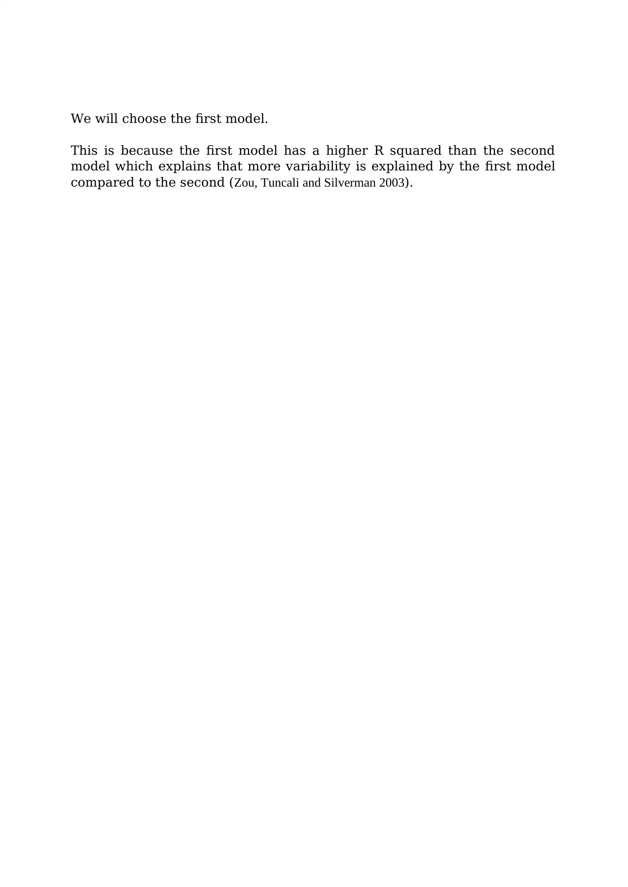
We will choose the first model.
This is because the first model has a higher R squared than the second
model which explains that more variability is explained by the first model
compared to the second (Zou, Tuncali and Silverman 2003).
This is because the first model has a higher R squared than the second
model which explains that more variability is explained by the first model
compared to the second (Zou, Tuncali and Silverman 2003).
Paraphrase This Document
Need a fresh take? Get an instant paraphrase of this document with our AI Paraphraser
Question 2:
Suppose are searcher wants to analysis the short-term interest rate and
she develops a model given by
i 3 inf t def t
where 𝒊𝟑𝒕 is the three-month T-bill rate, 𝒊𝒏𝒇𝒕 is the annual inflation rate based on the consumer
price index (CPI), and 𝒅𝒆𝒇𝒕 is the federal budget surplus or deficit as a percentage of GDP. He
collects the yearly data for the period from 1960 to 2016 (57 observations) from the Federal Reserve
Economic Data. They are in the Excel file Interest_rate.xlsx.
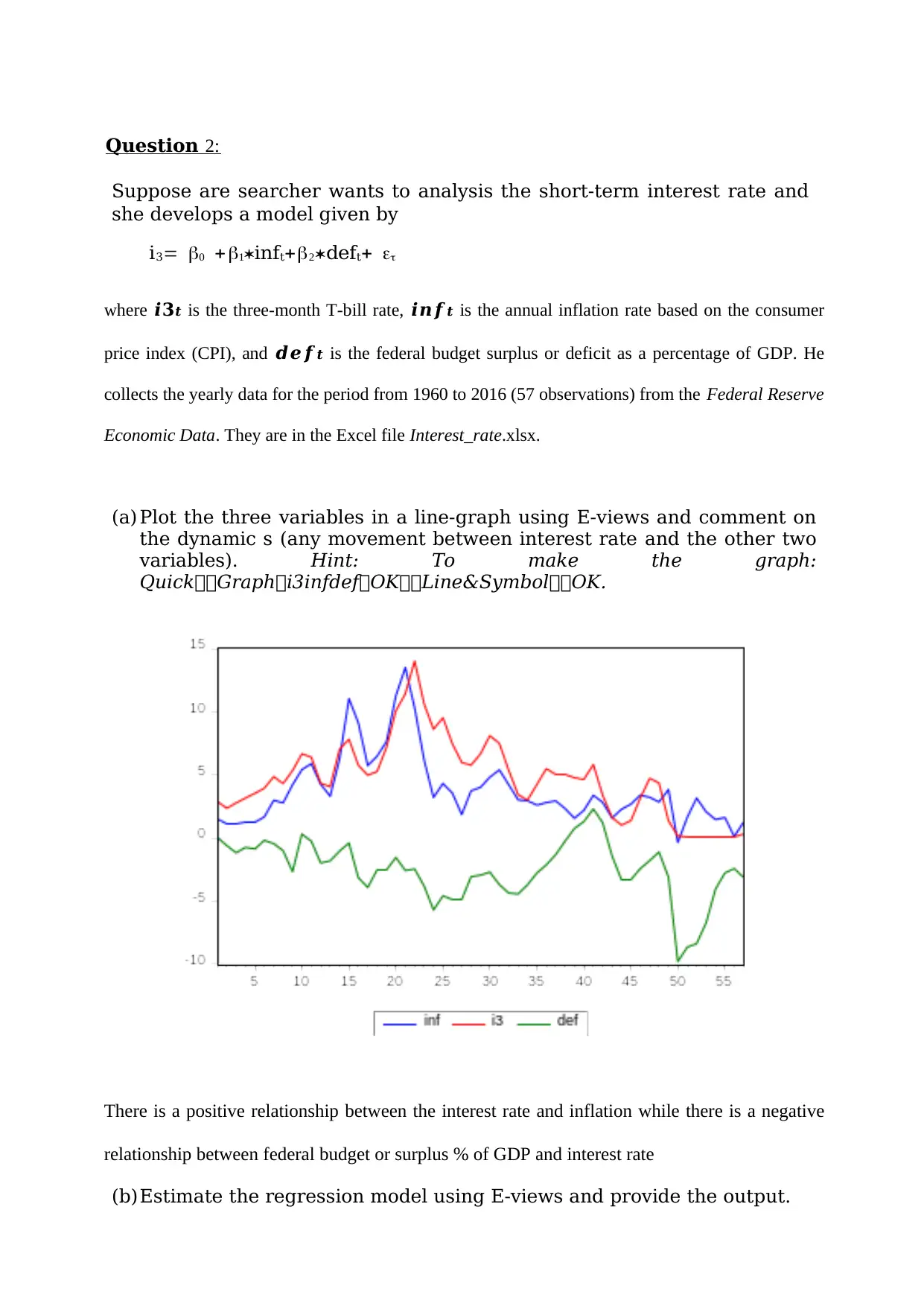
(a) Plot the three variables in a line-graph using E-views and comment on
the dynamic s (any movement between interest rate and the other two
variables). Hint: To make the graph:
QuickGraphi3infdefOKLine&SymbolOK.
There is a positive relationship between the interest rate and inflation while there is a negative
relationship between federal budget or surplus % of GDP and interest rate
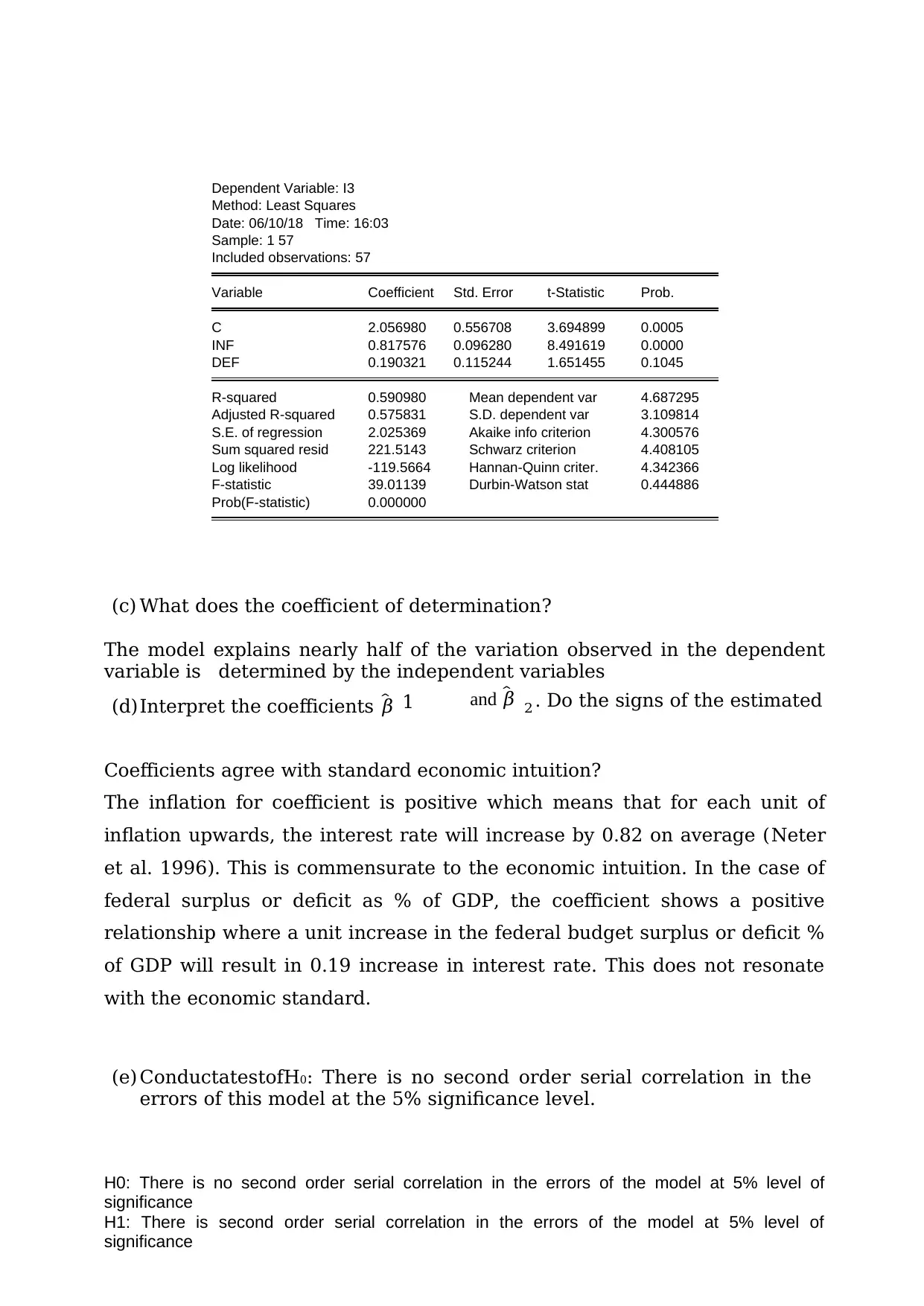
(b)Estimate the regression model using E-views and provide the output.
Suppose are searcher wants to analysis the short-term interest rate and
she develops a model given by
i 3 inf t def t
where 𝒊𝟑𝒕 is the three-month T-bill rate, 𝒊𝒏𝒇𝒕 is the annual inflation rate based on the consumer
price index (CPI), and 𝒅𝒆𝒇𝒕 is the federal budget surplus or deficit as a percentage of GDP. He
collects the yearly data for the period from 1960 to 2016 (57 observations) from the Federal Reserve
Economic Data. They are in the Excel file Interest_rate.xlsx.
(a) Plot the three variables in a line-graph using E-views and comment on
the dynamic s (any movement between interest rate and the other two
variables). Hint: To make the graph:
QuickGraphi3infdefOKLine&SymbolOK.
There is a positive relationship between the interest rate and inflation while there is a negative
relationship between federal budget or surplus % of GDP and interest rate
(b)Estimate the regression model using E-views and provide the output.
2
Dependent Variable: I3
Method: Least Squares
Date: 06/10/18 Time: 16:03
Sample: 1 57
Included observations: 57
Variable Coefficient Std. Error t-Statistic Prob.
C 2.056980 0.556708 3.694899 0.0005
INF 0.817576 0.096280 8.491619 0.0000
DEF 0.190321 0.115244 1.651455 0.1045
R-squared 0.590980 Mean dependent var 4.687295
Adjusted R-squared 0.575831 S.D. dependent var 3.109814
S.E. of regression 2.025369 Akaike info criterion 4.300576
Sum squared resid 221.5143 Schwarz criterion 4.408105
Log likelihood -119.5664 Hannan-Quinn criter. 4.342366
F-statistic 39.01139 Durbin-Watson stat 0.444886
Prob(F-statistic) 0.000000
(c) What does the coefficient of determination?
The model explains nearly half of the variation observed in the dependent
variable is determined by the independent variables
(d)Interpret the coefficients 𝛽̂ 1 and 𝛽̂ . Do the signs of the estimated
Coefficients agree with standard economic intuition?
The inflation for coefficient is positive which means that for each unit of
inflation upwards, the interest rate will increase by 0.82 on average (Neter
et al. 1996). This is commensurate to the economic intuition. In the case of
federal surplus or deficit as % of GDP, the coefficient shows a positive
relationship where a unit increase in the federal budget surplus or deficit %
of GDP will result in 0.19 increase in interest rate. This does not resonate
with the economic standard.
(e) ConductatestofH0: There is no second order serial correlation in the
errors of this model at the 5% significance level.
H0: There is no second order serial correlation in the errors of the model at 5% level of
significance
H1: There is second order serial correlation in the errors of the model at 5% level of
significance
⊘ This is a preview!⊘
Do you want full access?
Subscribe today to unlock all pages.
Trusted by 1+ million students worldwide
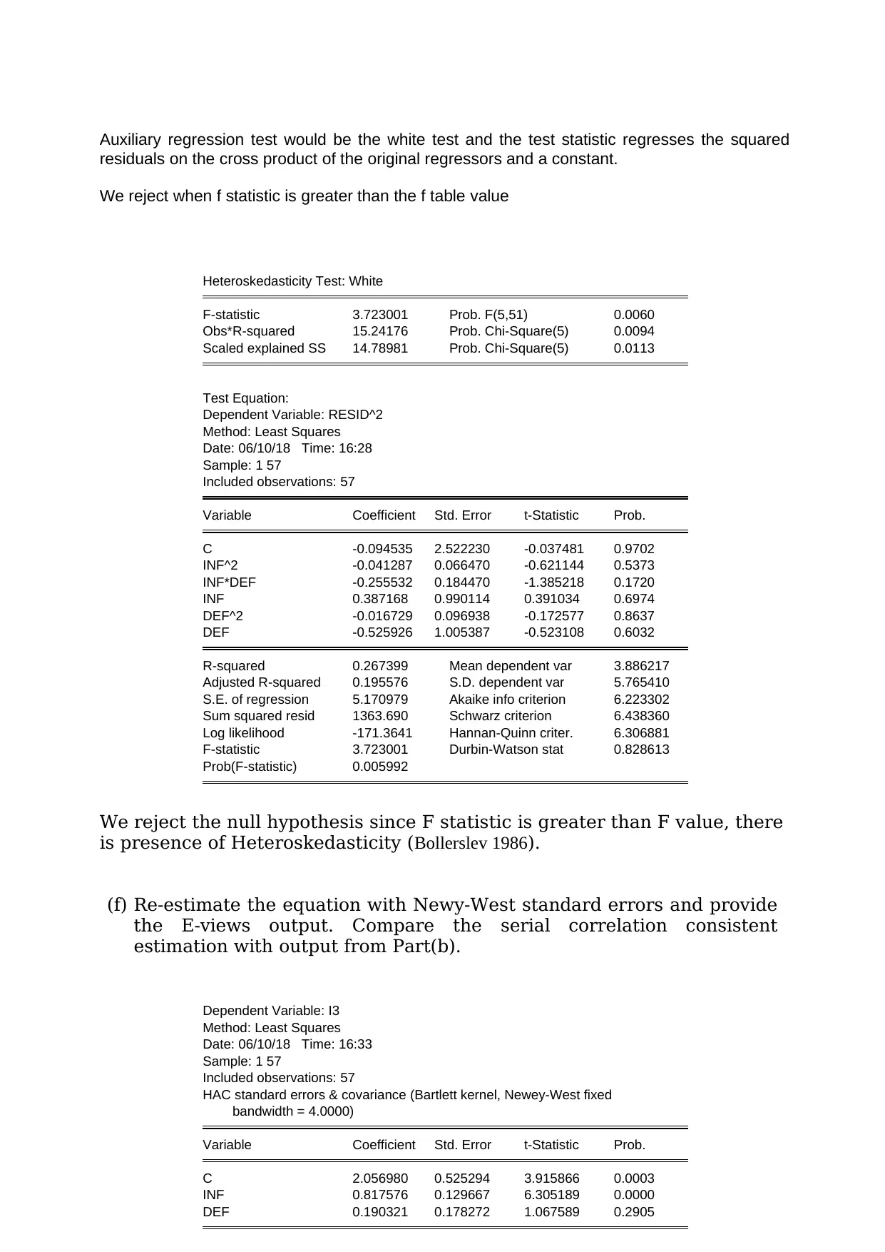
Auxiliary regression test would be the white test and the test statistic regresses the squared
residuals on the cross product of the original regressors and a constant.
We reject when f statistic is greater than the f table value
Heteroskedasticity Test: White
F-statistic 3.723001 Prob. F(5,51) 0.0060
Obs*R-squared 15.24176 Prob. Chi-Square(5) 0.0094
Scaled explained SS 14.78981 Prob. Chi-Square(5) 0.0113
Test Equation:
Dependent Variable: RESID^2
Method: Least Squares
Date: 06/10/18 Time: 16:28
Sample: 1 57
Included observations: 57
Variable Coefficient Std. Error t-Statistic Prob.
C -0.094535 2.522230 -0.037481 0.9702
INF^2 -0.041287 0.066470 -0.621144 0.5373
INF*DEF -0.255532 0.184470 -1.385218 0.1720
INF 0.387168 0.990114 0.391034 0.6974
DEF^2 -0.016729 0.096938 -0.172577 0.8637
DEF -0.525926 1.005387 -0.523108 0.6032
R-squared 0.267399 Mean dependent var 3.886217
Adjusted R-squared 0.195576 S.D. dependent var 5.765410
S.E. of regression 5.170979 Akaike info criterion 6.223302
Sum squared resid 1363.690 Schwarz criterion 6.438360
Log likelihood -171.3641 Hannan-Quinn criter. 6.306881
F-statistic 3.723001 Durbin-Watson stat 0.828613
Prob(F-statistic) 0.005992
We reject the null hypothesis since F statistic is greater than F value, there
is presence of Heteroskedasticity (Bollerslev 1986).
(f) Re-estimate the equation with Newy-West standard errors and provide
the E-views output. Compare the serial correlation consistent
estimation with output from Part(b).
Dependent Variable: I3
Method: Least Squares
Date: 06/10/18 Time: 16:33
Sample: 1 57
Included observations: 57
HAC standard errors & covariance (Bartlett kernel, Newey-West fixed
bandwidth = 4.0000)
Variable Coefficient Std. Error t-Statistic Prob.
C 2.056980 0.525294 3.915866 0.0003
INF 0.817576 0.129667 6.305189 0.0000
DEF 0.190321 0.178272 1.067589 0.2905
Paraphrase This Document
Need a fresh take? Get an instant paraphrase of this document with our AI Paraphraser
R-squared 0.590980 Mean dependent var 4.687295
Adjusted R-squared 0.575831 S.D. dependent var 3.109814
S.E. of regression 2.025369 Akaike info criterion 4.300576
Sum squared resid 221.5143 Schwarz criterion 4.408105
Log likelihood -119.5664 Hannan-Quinn criter. 4.342366
F-statistic 39.01139 Durbin-Watson stat 0.444886
Prob(F-statistic) 0.000000 Wald F-statistic 21.38973
Prob(Wald F-statistic) 0.000000
Heteroskedasticity Test: White
F-statistic 3.723001 Prob. F(5,51) 0.0060
Obs*R-squared 15.24176 Prob. Chi-Square(5) 0.0094
Scaled explained SS 14.78981 Prob. Chi-Square(5) 0.0113
Test Equation:
Dependent Variable: RESID^2
Method: Least Squares
Date: 06/10/18 Time: 16:34
Sample: 1 57
Included observations: 57
HAC standard errors & covariance (Bartlett kernel, Newey-West fixed
bandwidth = 4.0000)
Variable Coefficient Std. Error t-Statistic Prob.
C -0.094535 1.721952 -0.054900 0.9564
INF^2 -0.041287 0.075323 -0.548137 0.5860
INF*DEF -0.255532 0.230601 -1.108113 0.2730
INF 0.387168 0.770560 0.502450 0.6175
DEF^2 -0.016729 0.085688 -0.195234 0.8460
DEF -0.525926 0.832839 -0.631486 0.5305
R-squared 0.267399 Mean dependent var 3.886217
Adjusted R-squared 0.195576 S.D. dependent var 5.765410
S.E. of regression 5.170979 Akaike info criterion 6.223302
Sum squared resid 1363.690 Schwarz criterion 6.438360
Log likelihood -171.3641 Hannan-Quinn criter. 6.306881
F-statistic 3.723001 Durbin-Watson stat 0.828613
Prob(F-statistic) 0.005992
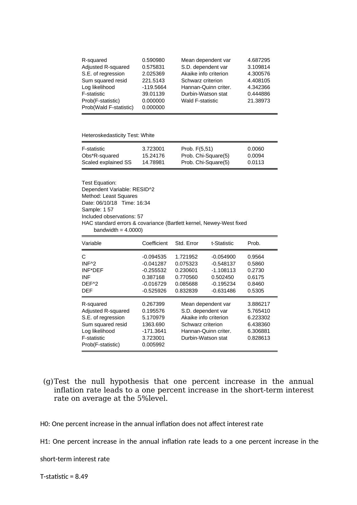
(g)Test the null hypothesis that one percent increase in the annual
inflation rate leads to a one percent increase in the short-term interest
rate on average at the 5%level.
H0: One percent increase in the annual inflation does not affect interest rate
H1: One percent increase in the annual inflation rate leads to a one percent increase in the
short-term interest rate
T-statistic = 8.49
Adjusted R-squared 0.575831 S.D. dependent var 3.109814
S.E. of regression 2.025369 Akaike info criterion 4.300576
Sum squared resid 221.5143 Schwarz criterion 4.408105
Log likelihood -119.5664 Hannan-Quinn criter. 4.342366
F-statistic 39.01139 Durbin-Watson stat 0.444886
Prob(F-statistic) 0.000000 Wald F-statistic 21.38973
Prob(Wald F-statistic) 0.000000
Heteroskedasticity Test: White
F-statistic 3.723001 Prob. F(5,51) 0.0060
Obs*R-squared 15.24176 Prob. Chi-Square(5) 0.0094
Scaled explained SS 14.78981 Prob. Chi-Square(5) 0.0113
Test Equation:
Dependent Variable: RESID^2
Method: Least Squares
Date: 06/10/18 Time: 16:34
Sample: 1 57
Included observations: 57
HAC standard errors & covariance (Bartlett kernel, Newey-West fixed
bandwidth = 4.0000)
Variable Coefficient Std. Error t-Statistic Prob.
C -0.094535 1.721952 -0.054900 0.9564
INF^2 -0.041287 0.075323 -0.548137 0.5860
INF*DEF -0.255532 0.230601 -1.108113 0.2730
INF 0.387168 0.770560 0.502450 0.6175
DEF^2 -0.016729 0.085688 -0.195234 0.8460
DEF -0.525926 0.832839 -0.631486 0.5305
R-squared 0.267399 Mean dependent var 3.886217
Adjusted R-squared 0.195576 S.D. dependent var 5.765410
S.E. of regression 5.170979 Akaike info criterion 6.223302
Sum squared resid 1363.690 Schwarz criterion 6.438360
Log likelihood -171.3641 Hannan-Quinn criter. 6.306881
F-statistic 3.723001 Durbin-Watson stat 0.828613
Prob(F-statistic) 0.005992
(g)Test the null hypothesis that one percent increase in the annual
inflation rate leads to a one percent increase in the short-term interest
rate on average at the 5%level.
H0: One percent increase in the annual inflation does not affect interest rate
H1: One percent increase in the annual inflation rate leads to a one percent increase in the
short-term interest rate
T-statistic = 8.49

T-table value = 1.673034
Since the t-critical value is less than the t-statistic we reject the null hypothesis.
Since the t-critical value is less than the t-statistic we reject the null hypothesis.
⊘ This is a preview!⊘
Do you want full access?
Subscribe today to unlock all pages.
Trusted by 1+ million students worldwide
Question 3:
In the file pubexp.xls there are data on public expenditure on
education(EE), gross domestic product(GDP) and population(P) for 34
countries in theyear1980.Itishypothesizedthatpercapita expenditure on
education is linearly related to per capita GDP. That is-
yi12xii
wher
e
V=E
Ei Pi
and
GDPi.P xi
In the file pubexp.xls there are data on public expenditure on
education(EE), gross domestic product(GDP) and population(P) for 34
countries in theyear1980.Itishypothesizedthatpercapita expenditure on
education is linearly related to per capita GDP. That is-
yi12xii
wher
e
V=E
Ei Pi
and
GDPi.P xi
Paraphrase This Document
Need a fresh take? Get an instant paraphrase of this document with our AI Paraphraser
RESEARCH ON PHYSICAL AGGRESSION
i i
Import the data into E-views.
(a) Issues suspected that𝜀𝑖 may be heteroskedastic with a variance
related to𝑥.
(b)Why might the suspicion about heteroskedasticity be reasonable?
There is a positive relationship for the error term and the x variable.
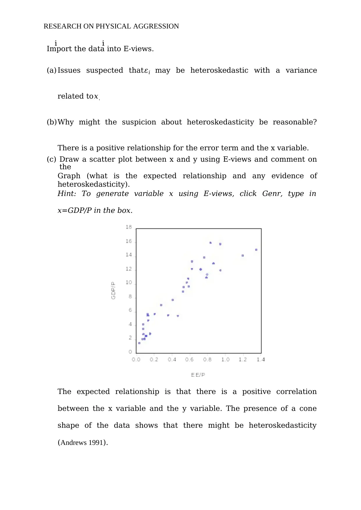
(c) Draw a scatter plot between x and y using E-views and comment on
the
Graph (what is the expected relationship and any evidence of
heteroskedasticity).
Hint: To generate variable x using E-views, click Genr, type in
x=GDP/P in the box.
The expected relationship is that there is a positive correlation
between the x variable and the y variable. The presence of a cone
shape of the data shows that there might be heteroskedasticity
(Andrews 1991).
i i
Import the data into E-views.
(a) Issues suspected that𝜀𝑖 may be heteroskedastic with a variance
related to𝑥.
(b)Why might the suspicion about heteroskedasticity be reasonable?
There is a positive relationship for the error term and the x variable.
(c) Draw a scatter plot between x and y using E-views and comment on
the
Graph (what is the expected relationship and any evidence of
heteroskedasticity).
Hint: To generate variable x using E-views, click Genr, type in
x=GDP/P in the box.
The expected relationship is that there is a positive correlation
between the x variable and the y variable. The presence of a cone
shape of the data shows that there might be heteroskedasticity
(Andrews 1991).
1RESEARCH ON PHYSICAL AGGRESSION
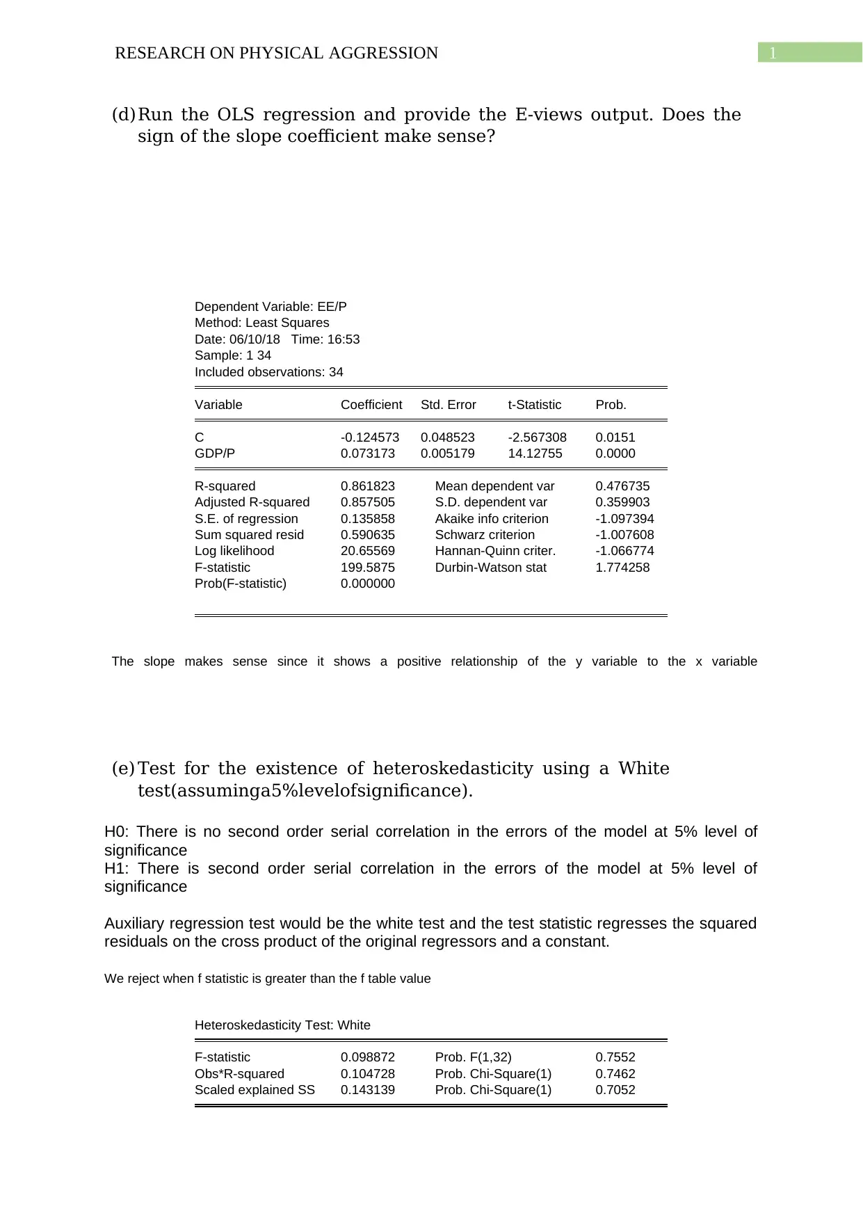
(d)Run the OLS regression and provide the E-views output. Does the
sign of the slope coefficient make sense?
Dependent Variable: EE/P
Method: Least Squares
Date: 06/10/18 Time: 16:53
Sample: 1 34
Included observations: 34
Variable Coefficient Std. Error t-Statistic Prob.
C -0.124573 0.048523 -2.567308 0.0151
GDP/P 0.073173 0.005179 14.12755 0.0000
R-squared 0.861823 Mean dependent var 0.476735
Adjusted R-squared 0.857505 S.D. dependent var 0.359903
S.E. of regression 0.135858 Akaike info criterion -1.097394
Sum squared resid 0.590635 Schwarz criterion -1.007608
Log likelihood 20.65569 Hannan-Quinn criter. -1.066774
F-statistic 199.5875 Durbin-Watson stat 1.774258
Prob(F-statistic) 0.000000
The slope makes sense since it shows a positive relationship of the y variable to the x variable
(e) Test for the existence of heteroskedasticity using a White
test(assuminga5%levelofsignificance).
H0: There is no second order serial correlation in the errors of the model at 5% level of
significance
H1: There is second order serial correlation in the errors of the model at 5% level of
significance
Auxiliary regression test would be the white test and the test statistic regresses the squared
residuals on the cross product of the original regressors and a constant.
We reject when f statistic is greater than the f table value
Heteroskedasticity Test: White
F-statistic 0.098872 Prob. F(1,32) 0.7552
Obs*R-squared 0.104728 Prob. Chi-Square(1) 0.7462
Scaled explained SS 0.143139 Prob. Chi-Square(1) 0.7052
⊘ This is a preview!⊘
Do you want full access?
Subscribe today to unlock all pages.
Trusted by 1+ million students worldwide
1 out of 15
Related Documents


Your All-in-One AI-Powered Toolkit for Academic Success.
+13062052269
info@desklib.com
Available 24*7 on WhatsApp / Email
![[object Object]](/_next/static/media/star-bottom.7253800d.svg)
Unlock your academic potential
Copyright © 2020–2026 A2Z Services. All Rights Reserved. Developed and managed by ZUCOL.