Econometrics and Business Statistics: Solved Homework Problems
VerifiedAdded on 2023/06/12
|15
|2830
|124
Homework Assignment
AI Summary
This assignment solution covers various aspects of econometrics and business statistics. It includes regression analysis, hypothesis testing, and addressing issues like serial correlation and heteroskedasticity. The first question focuses on interpreting regression output related to student math scores and school expenditures, including testing the significance of variables like lunch program participation. The second question examines the relationship between Treasury bill rates, inflation, and federal budget deficits, incorporating tests for serial autocorrelation and using Newey-West standard errors. The third question discusses heteroskedasticity in the context of per capita GDP and education expenditure, including OLS regression analysis and addressing potential violations of assumptions. This detailed solution offers insights into applying econometric techniques to real-world problems. Desklib provides access to similar solved assignments and past papers for students.
Running Head: ECONOMETRICS AND BUSINESS STATISTICS
ECONOMETRICS AND BUSINESS STATISTICS
Name of the Student
Name of the University
Author Note
ECONOMETRICS AND BUSINESS STATISTICS
Name of the Student
Name of the University
Author Note
Paraphrase This Document
Need a fresh take? Get an instant paraphrase of this document with our AI Paraphraser
1ECONOMETRICS AND BUSINESS STATISTICS
Table of Contents
Answer 1..........................................................................................................................................3
Answer a......................................................................................................................................3
Answer b......................................................................................................................................3
Answer c......................................................................................................................................4
Answer d......................................................................................................................................4
Answer e......................................................................................................................................4
Answer 2..........................................................................................................................................5
Answer a......................................................................................................................................5
Answer b......................................................................................................................................6
Answer c......................................................................................................................................6
Answer d......................................................................................................................................7
Answer e......................................................................................................................................7
Part f.............................................................................................................................................9
Part g..........................................................................................................................................10
Answer 3........................................................................................................................................11
Answer a....................................................................................................................................11
Answer b....................................................................................................................................11
Answer c....................................................................................................................................12
Answer d....................................................................................................................................13
Answer e....................................................................................................................................14
Answer f.....................................................................................................................................15
2ECONOMETRICS AND BUSINESS STATISTICS
Answer 1
Answer a
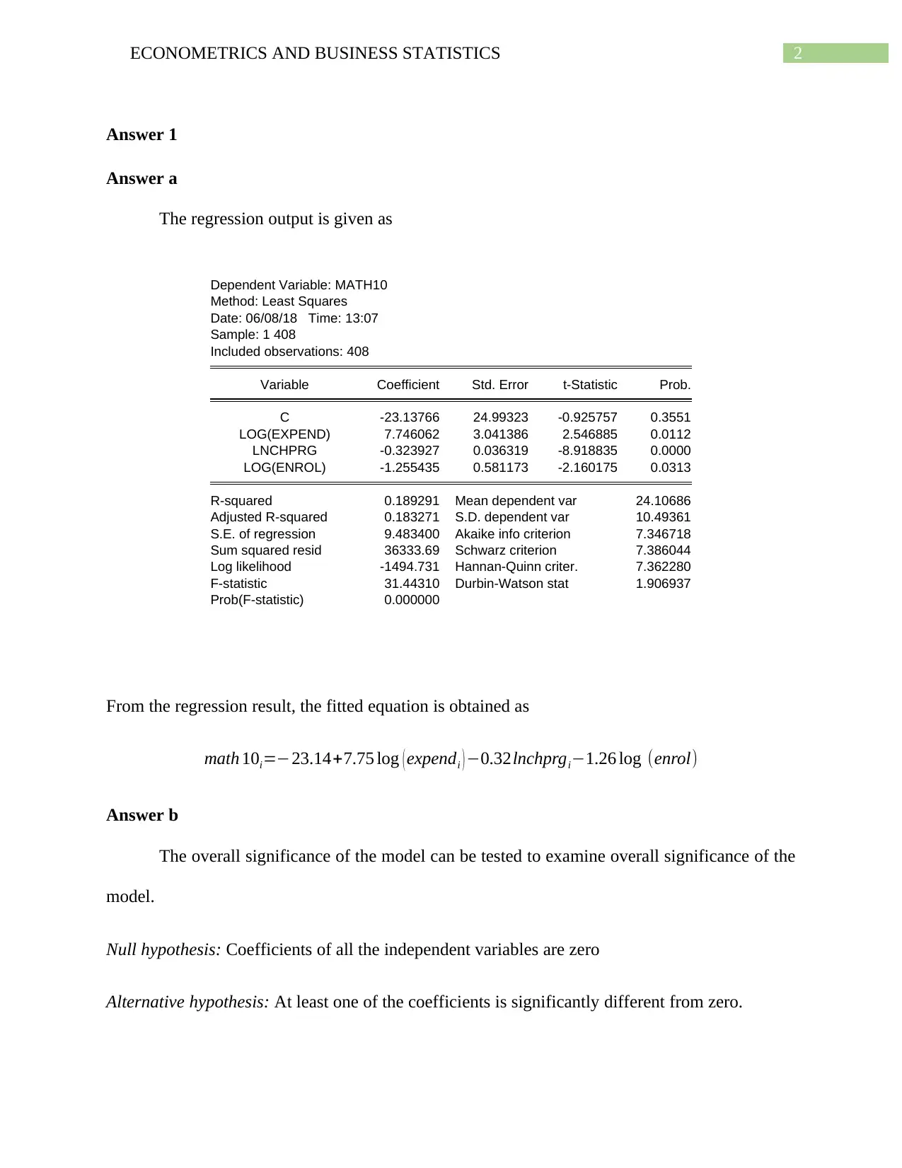
The regression output is given as
Dependent Variable: MATH10
Method: Least Squares
Date: 06/08/18 Time: 13:07
Sample: 1 408
Included observations: 408
Variable Coefficient Std. Error t-Statistic Prob.
C -23.13766 24.99323 -0.925757 0.3551
LOG(EXPEND) 7.746062 3.041386 2.546885 0.0112
LNCHPRG -0.323927 0.036319 -8.918835 0.0000
LOG(ENROL) -1.255435 0.581173 -2.160175 0.0313
R-squared 0.189291 Mean dependent var 24.10686
Adjusted R-squared 0.183271 S.D. dependent var 10.49361
S.E. of regression 9.483400 Akaike info criterion 7.346718
Sum squared resid 36333.69 Schwarz criterion 7.386044
Log likelihood -1494.731 Hannan-Quinn criter. 7.362280
F-statistic 31.44310 Durbin-Watson stat 1.906937
Prob(F-statistic) 0.000000
From the regression result, the fitted equation is obtained as
math 10i=−23.14+7.75 log ( expendi ) −0.32lnchprgi−1.26 log (enrol)
Answer b
The overall significance of the model can be tested to examine overall significance of the
model.
Null hypothesis: Coefficients of all the independent variables are zero
Alternative hypothesis: At least one of the coefficients is significantly different from zero.
Answer 1
Answer a
The regression output is given as
Dependent Variable: MATH10
Method: Least Squares
Date: 06/08/18 Time: 13:07
Sample: 1 408
Included observations: 408
Variable Coefficient Std. Error t-Statistic Prob.
C -23.13766 24.99323 -0.925757 0.3551
LOG(EXPEND) 7.746062 3.041386 2.546885 0.0112
LNCHPRG -0.323927 0.036319 -8.918835 0.0000
LOG(ENROL) -1.255435 0.581173 -2.160175 0.0313
R-squared 0.189291 Mean dependent var 24.10686
Adjusted R-squared 0.183271 S.D. dependent var 10.49361
S.E. of regression 9.483400 Akaike info criterion 7.346718
Sum squared resid 36333.69 Schwarz criterion 7.386044
Log likelihood -1494.731 Hannan-Quinn criter. 7.362280
F-statistic 31.44310 Durbin-Watson stat 1.906937
Prob(F-statistic) 0.000000
From the regression result, the fitted equation is obtained as
math 10i=−23.14+7.75 log ( expendi ) −0.32lnchprgi−1.26 log (enrol)
Answer b
The overall significance of the model can be tested to examine overall significance of the
model.
Null hypothesis: Coefficients of all the independent variables are zero
Alternative hypothesis: At least one of the coefficients is significantly different from zero.
⊘ This is a preview!⊘
Do you want full access?
Subscribe today to unlock all pages.
Trusted by 1+ million students worldwide
3ECONOMETRICS AND BUSINESS STATISTICS
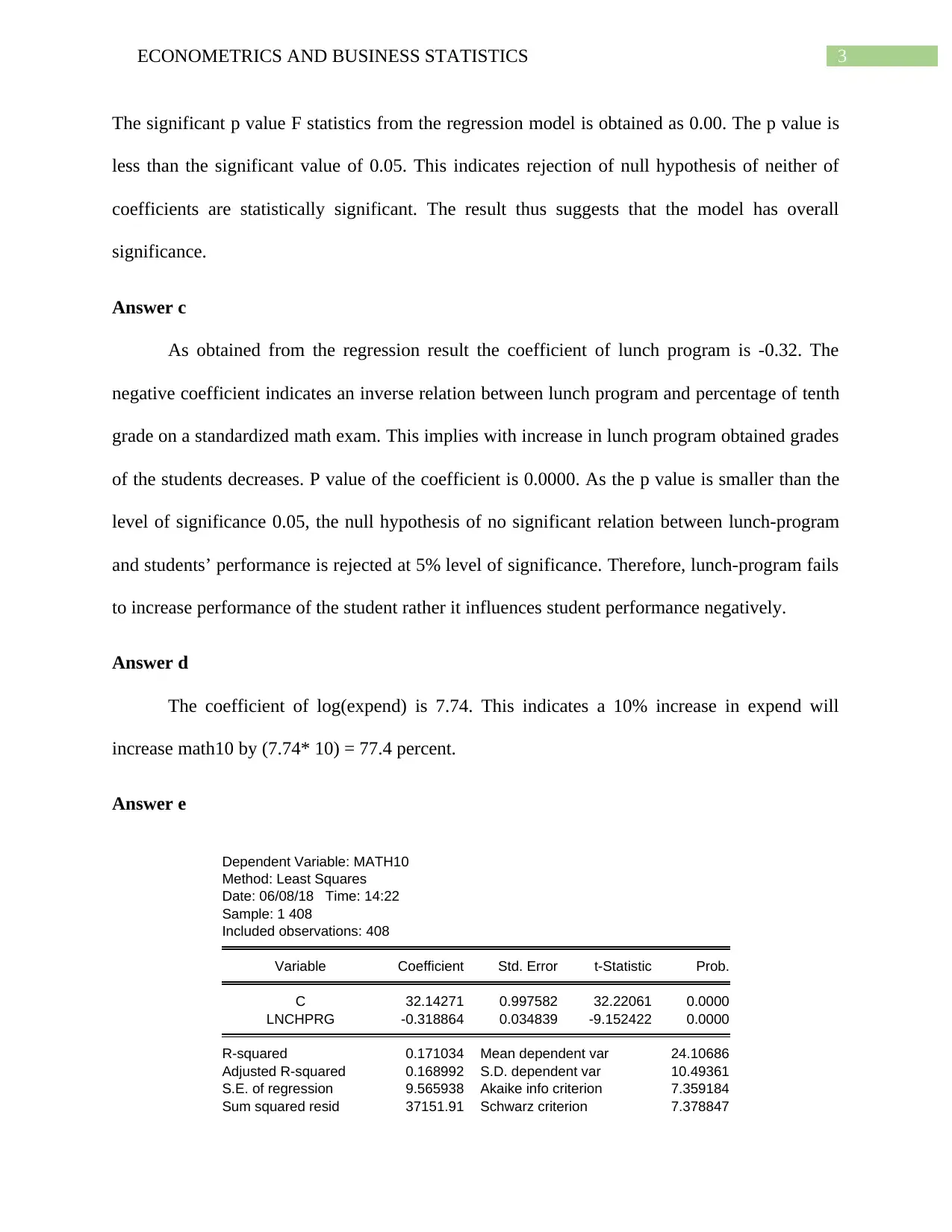
The significant p value F statistics from the regression model is obtained as 0.00. The p value is
less than the significant value of 0.05. This indicates rejection of null hypothesis of neither of
coefficients are statistically significant. The result thus suggests that the model has overall
significance.
Answer c
As obtained from the regression result the coefficient of lunch program is -0.32. The
negative coefficient indicates an inverse relation between lunch program and percentage of tenth
grade on a standardized math exam. This implies with increase in lunch program obtained grades
of the students decreases. P value of the coefficient is 0.0000. As the p value is smaller than the
level of significance 0.05, the null hypothesis of no significant relation between lunch-program
and students’ performance is rejected at 5% level of significance. Therefore, lunch-program fails
to increase performance of the student rather it influences student performance negatively.
Answer d
The coefficient of log(expend) is 7.74. This indicates a 10% increase in expend will
increase math10 by (7.74* 10) = 77.4 percent.
Answer e
Dependent Variable: MATH10
Method: Least Squares
Date: 06/08/18 Time: 14:22
Sample: 1 408
Included observations: 408
Variable Coefficient Std. Error t-Statistic Prob.
C 32.14271 0.997582 32.22061 0.0000
LNCHPRG -0.318864 0.034839 -9.152422 0.0000
R-squared 0.171034 Mean dependent var 24.10686
Adjusted R-squared 0.168992 S.D. dependent var 10.49361
S.E. of regression 9.565938 Akaike info criterion 7.359184
Sum squared resid 37151.91 Schwarz criterion 7.378847
Paraphrase This Document
Need a fresh take? Get an instant paraphrase of this document with our AI Paraphraser
4ECONOMETRICS AND BUSINESS STATISTICS
Log likelihood -1499.274 Hannan-Quinn criter. 7.366965
F-statistic 83.76683 Durbin-Watson stat 1.907745
Prob(F-statistic) 0.000000
In both the model, the variable lunch program is negative and statistically significant. The
magnitude of the coefficient in both the model is equivalent to -0.32. For the model in part (a)
the value of adjusted R square is 0.18. In the new model, the R square value is 0.16. The R
square value indicates goodness of fit of the model. This explains how much variation in the
dependent variable is explained by the independent variable. Higher the R square value better is
fitted model. In terms of R square value, model 1 is more acceptable as compared to model 2.
Answer 2
Answer a
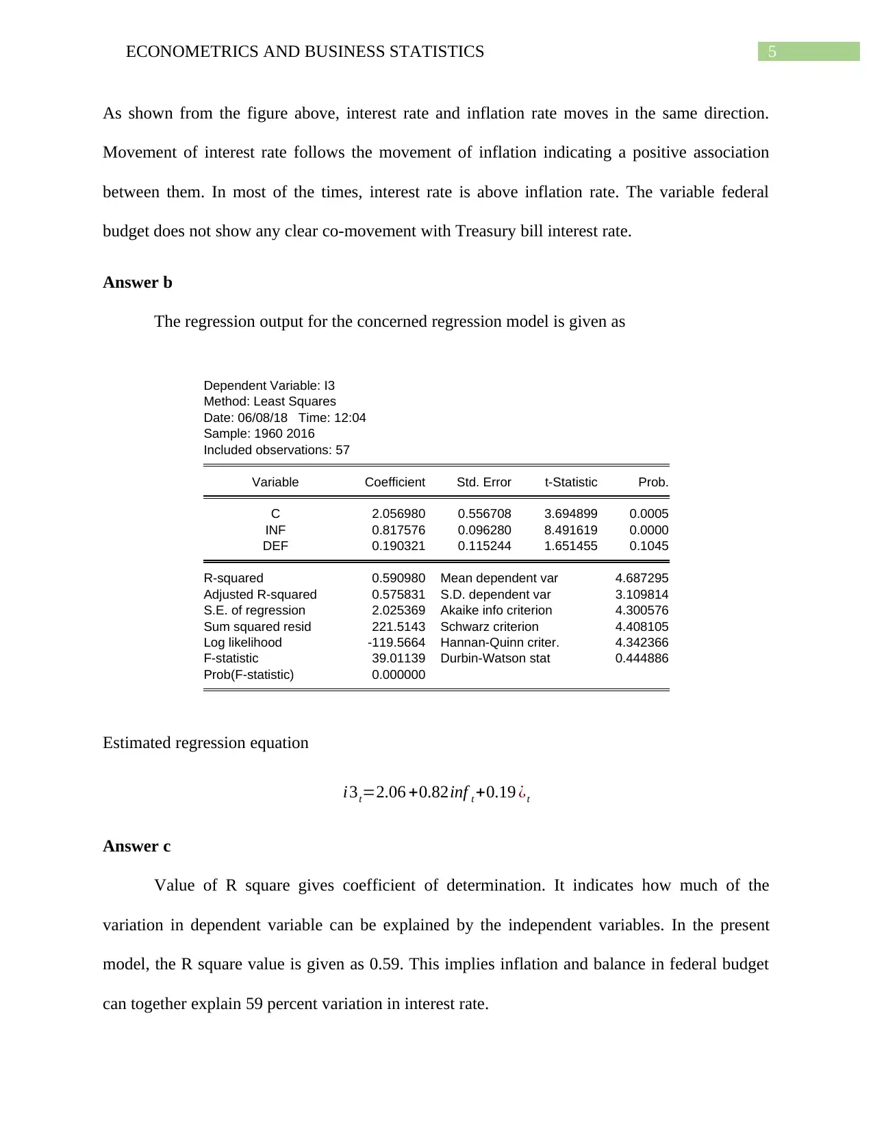
Figure 1: Line plot of T-bill rate, inflation rate and federal budget balance
Log likelihood -1499.274 Hannan-Quinn criter. 7.366965
F-statistic 83.76683 Durbin-Watson stat 1.907745
Prob(F-statistic) 0.000000
In both the model, the variable lunch program is negative and statistically significant. The
magnitude of the coefficient in both the model is equivalent to -0.32. For the model in part (a)
the value of adjusted R square is 0.18. In the new model, the R square value is 0.16. The R
square value indicates goodness of fit of the model. This explains how much variation in the
dependent variable is explained by the independent variable. Higher the R square value better is
fitted model. In terms of R square value, model 1 is more acceptable as compared to model 2.
Answer 2
Answer a
Figure 1: Line plot of T-bill rate, inflation rate and federal budget balance
5ECONOMETRICS AND BUSINESS STATISTICS
As shown from the figure above, interest rate and inflation rate moves in the same direction.
Movement of interest rate follows the movement of inflation indicating a positive association
between them. In most of the times, interest rate is above inflation rate. The variable federal
budget does not show any clear co-movement with Treasury bill interest rate.
Answer b
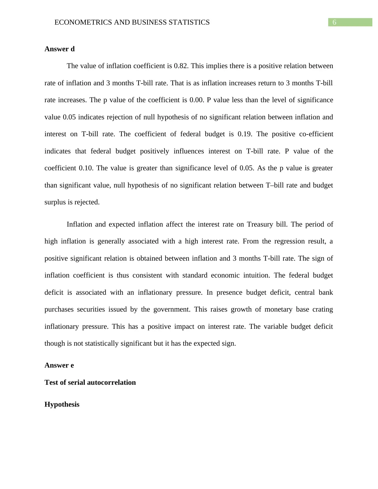
The regression output for the concerned regression model is given as
Dependent Variable: I3
Method: Least Squares
Date: 06/08/18 Time: 12:04
Sample: 1960 2016
Included observations: 57
Variable Coefficient Std. Error t-Statistic Prob.
C 2.056980 0.556708 3.694899 0.0005
INF 0.817576 0.096280 8.491619 0.0000
DEF 0.190321 0.115244 1.651455 0.1045
R-squared 0.590980 Mean dependent var 4.687295
Adjusted R-squared 0.575831 S.D. dependent var 3.109814
S.E. of regression 2.025369 Akaike info criterion 4.300576
Sum squared resid 221.5143 Schwarz criterion 4.408105
Log likelihood -119.5664 Hannan-Quinn criter. 4.342366
F-statistic 39.01139 Durbin-Watson stat 0.444886
Prob(F-statistic) 0.000000
Estimated regression equation
i3t=2.06 +0.82inf t +0.19 ¿t
Answer c
Value of R square gives coefficient of determination. It indicates how much of the
variation in dependent variable can be explained by the independent variables. In the present
model, the R square value is given as 0.59. This implies inflation and balance in federal budget
can together explain 59 percent variation in interest rate.
As shown from the figure above, interest rate and inflation rate moves in the same direction.
Movement of interest rate follows the movement of inflation indicating a positive association
between them. In most of the times, interest rate is above inflation rate. The variable federal
budget does not show any clear co-movement with Treasury bill interest rate.
Answer b
The regression output for the concerned regression model is given as
Dependent Variable: I3
Method: Least Squares
Date: 06/08/18 Time: 12:04
Sample: 1960 2016
Included observations: 57
Variable Coefficient Std. Error t-Statistic Prob.
C 2.056980 0.556708 3.694899 0.0005
INF 0.817576 0.096280 8.491619 0.0000
DEF 0.190321 0.115244 1.651455 0.1045
R-squared 0.590980 Mean dependent var 4.687295
Adjusted R-squared 0.575831 S.D. dependent var 3.109814
S.E. of regression 2.025369 Akaike info criterion 4.300576
Sum squared resid 221.5143 Schwarz criterion 4.408105
Log likelihood -119.5664 Hannan-Quinn criter. 4.342366
F-statistic 39.01139 Durbin-Watson stat 0.444886
Prob(F-statistic) 0.000000
Estimated regression equation
i3t=2.06 +0.82inf t +0.19 ¿t
Answer c
Value of R square gives coefficient of determination. It indicates how much of the
variation in dependent variable can be explained by the independent variables. In the present
model, the R square value is given as 0.59. This implies inflation and balance in federal budget
can together explain 59 percent variation in interest rate.
⊘ This is a preview!⊘
Do you want full access?
Subscribe today to unlock all pages.
Trusted by 1+ million students worldwide
6ECONOMETRICS AND BUSINESS STATISTICS
Answer d
The value of inflation coefficient is 0.82. This implies there is a positive relation between
rate of inflation and 3 months T-bill rate. That is as inflation increases return to 3 months T-bill
rate increases. The p value of the coefficient is 0.00. P value less than the level of significance
value 0.05 indicates rejection of null hypothesis of no significant relation between inflation and
interest on T-bill rate. The coefficient of federal budget is 0.19. The positive co-efficient
indicates that federal budget positively influences interest on T-bill rate. P value of the
coefficient 0.10. The value is greater than significance level of 0.05. As the p value is greater
than significant value, null hypothesis of no significant relation between T–bill rate and budget
surplus is rejected.
Inflation and expected inflation affect the interest rate on Treasury bill. The period of
high inflation is generally associated with a high interest rate. From the regression result, a
positive significant relation is obtained between inflation and 3 months T-bill rate. The sign of
inflation coefficient is thus consistent with standard economic intuition. The federal budget
deficit is associated with an inflationary pressure. In presence budget deficit, central bank
purchases securities issued by the government. This raises growth of monetary base crating
inflationary pressure. This has a positive impact on interest rate. The variable budget deficit
though is not statistically significant but it has the expected sign.
Answer e
Test of serial autocorrelation
Hypothesis
Paraphrase This Document
Need a fresh take? Get an instant paraphrase of this document with our AI Paraphraser
7ECONOMETRICS AND BUSINESS STATISTICS
Null hypothesis: There is no second order serial autocorrelation in the model at 5% level of
significance
Alternative hypothesis: There exists a second order serial autocorrelation in the model at 5%
level of significance.
Auxiliary regression
The auxiliary regression regress current values of residuals on all the explanatory
variables and is related with lagged residual terms. The Breusch- Godfrey test statistics is given
as (T – p)*R2 , where T is the number of observation and p is the number of lagged residual
terms. The test statistics follows a chi-square distribution with p degrees of freedom.
Decision rule
The null hypothesis is rejected if P value of the Breusch-Godfrey test statistics is less
than 0.05.
Conclusion
From the test result, p value of the LM statistics is obtained as 0.0000. As the p value is
less than 0.05, the null hypothesis of no second order serial autocorrelation exists in the model is
rejected. This implies the model has the problem of second order autocorrelation.
8ECONOMETRICS AND BUSINESS STATISTICS
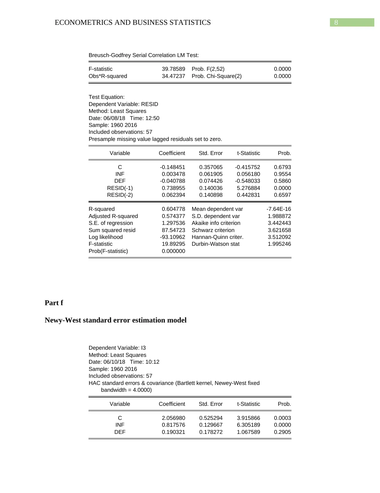
Breusch-Godfrey Serial Correlation LM Test:
F-statistic 39.78589 Prob. F(2,52) 0.0000
Obs*R-squared 34.47237 Prob. Chi-Square(2) 0.0000
Test Equation:
Dependent Variable: RESID
Method: Least Squares
Date: 06/08/18 Time: 12:50
Sample: 1960 2016
Included observations: 57
Presample missing value lagged residuals set to zero.
Variable Coefficient Std. Error t-Statistic Prob.
C -0.148451 0.357065 -0.415752 0.6793
INF 0.003478 0.061905 0.056180 0.9554
DEF -0.040788 0.074426 -0.548033 0.5860
RESID(-1) 0.738955 0.140036 5.276884 0.0000
RESID(-2) 0.062394 0.140898 0.442831 0.6597
R-squared 0.604778 Mean dependent var -7.64E-16
Adjusted R-squared 0.574377 S.D. dependent var 1.988872
S.E. of regression 1.297536 Akaike info criterion 3.442443
Sum squared resid 87.54723 Schwarz criterion 3.621658
Log likelihood -93.10962 Hannan-Quinn criter. 3.512092
F-statistic 19.89295 Durbin-Watson stat 1.995246
Prob(F-statistic) 0.000000
Part f
Newy-West standard error estimation model
Dependent Variable: I3
Method: Least Squares
Date: 06/10/18 Time: 10:12
Sample: 1960 2016
Included observations: 57
HAC standard errors & covariance (Bartlett kernel, Newey-West fixed
bandwidth = 4.0000)
Variable Coefficient Std. Error t-Statistic Prob.
C 2.056980 0.525294 3.915866 0.0003
INF 0.817576 0.129667 6.305189 0.0000
DEF 0.190321 0.178272 1.067589 0.2905
⊘ This is a preview!⊘
Do you want full access?
Subscribe today to unlock all pages.
Trusted by 1+ million students worldwide
9ECONOMETRICS AND BUSINESS STATISTICS
R-squared 0.590980 Mean dependent var 4.687295
Adjusted R-squared 0.575831 S.D. dependent var 3.109814
S.E. of regression 2.025369 Akaike info criterion 4.300576
Sum squared resid 221.5143 Schwarz criterion 4.408105
Log likelihood -119.5664 Hannan-Quinn criter. 4.342366
F-statistic 39.01139 Durbin-Watson stat 0.444886
Prob(F-statistic) 0.000000 Wald F-statistic 21.38973
Prob(Wald F-statistic) 0.000000
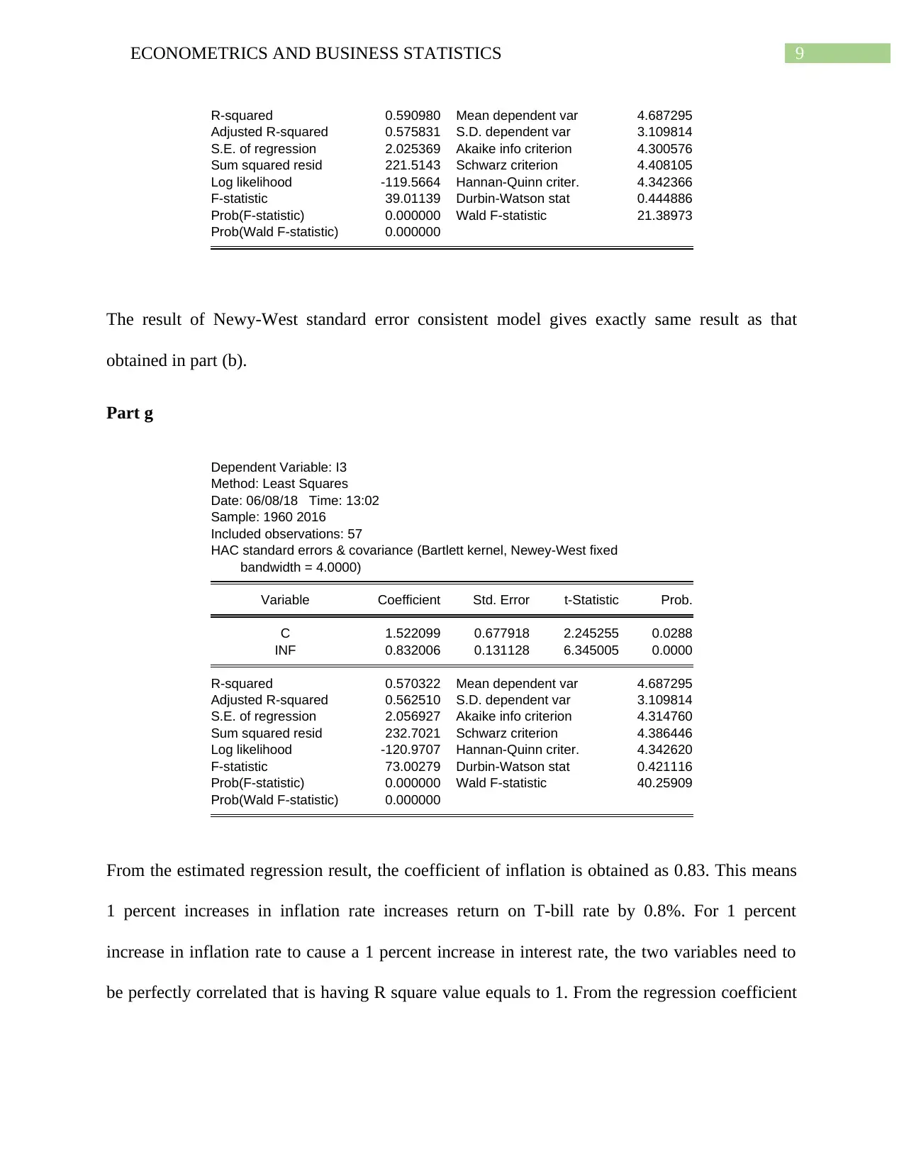
The result of Newy-West standard error consistent model gives exactly same result as that
obtained in part (b).
Part g
Dependent Variable: I3
Method: Least Squares
Date: 06/08/18 Time: 13:02
Sample: 1960 2016
Included observations: 57
HAC standard errors & covariance (Bartlett kernel, Newey-West fixed
bandwidth = 4.0000)
Variable Coefficient Std. Error t-Statistic Prob.
C 1.522099 0.677918 2.245255 0.0288
INF 0.832006 0.131128 6.345005 0.0000
R-squared 0.570322 Mean dependent var 4.687295
Adjusted R-squared 0.562510 S.D. dependent var 3.109814
S.E. of regression 2.056927 Akaike info criterion 4.314760
Sum squared resid 232.7021 Schwarz criterion 4.386446
Log likelihood -120.9707 Hannan-Quinn criter. 4.342620
F-statistic 73.00279 Durbin-Watson stat 0.421116
Prob(F-statistic) 0.000000 Wald F-statistic 40.25909
Prob(Wald F-statistic) 0.000000
From the estimated regression result, the coefficient of inflation is obtained as 0.83. This means
1 percent increases in inflation rate increases return on T-bill rate by 0.8%. For 1 percent
increase in inflation rate to cause a 1 percent increase in interest rate, the two variables need to
be perfectly correlated that is having R square value equals to 1. From the regression coefficient
R-squared 0.590980 Mean dependent var 4.687295
Adjusted R-squared 0.575831 S.D. dependent var 3.109814
S.E. of regression 2.025369 Akaike info criterion 4.300576
Sum squared resid 221.5143 Schwarz criterion 4.408105
Log likelihood -119.5664 Hannan-Quinn criter. 4.342366
F-statistic 39.01139 Durbin-Watson stat 0.444886
Prob(F-statistic) 0.000000 Wald F-statistic 21.38973
Prob(Wald F-statistic) 0.000000
The result of Newy-West standard error consistent model gives exactly same result as that
obtained in part (b).
Part g
Dependent Variable: I3
Method: Least Squares
Date: 06/08/18 Time: 13:02
Sample: 1960 2016
Included observations: 57
HAC standard errors & covariance (Bartlett kernel, Newey-West fixed
bandwidth = 4.0000)
Variable Coefficient Std. Error t-Statistic Prob.
C 1.522099 0.677918 2.245255 0.0288
INF 0.832006 0.131128 6.345005 0.0000
R-squared 0.570322 Mean dependent var 4.687295
Adjusted R-squared 0.562510 S.D. dependent var 3.109814
S.E. of regression 2.056927 Akaike info criterion 4.314760
Sum squared resid 232.7021 Schwarz criterion 4.386446
Log likelihood -120.9707 Hannan-Quinn criter. 4.342620
F-statistic 73.00279 Durbin-Watson stat 0.421116
Prob(F-statistic) 0.000000 Wald F-statistic 40.25909
Prob(Wald F-statistic) 0.000000
From the estimated regression result, the coefficient of inflation is obtained as 0.83. This means
1 percent increases in inflation rate increases return on T-bill rate by 0.8%. For 1 percent
increase in inflation rate to cause a 1 percent increase in interest rate, the two variables need to
be perfectly correlated that is having R square value equals to 1. From the regression coefficient
Paraphrase This Document
Need a fresh take? Get an instant paraphrase of this document with our AI Paraphraser
10ECONOMETRICS AND BUSINESS STATISTICS
and value of R square, the null hypothesis that 1 percent increase in inflation leads to a 1 percent
increase in interest rate is rejected.
Answer 3
Answer a
The suspicion about heteroskadascity is reasonable as countries with a higher per capita
GDP have access to a large amount of money to distribute. The people with a higher average
income enjoy a higher flexibility regarding their spending on education. Countries with smaller
per capita GDP has limited option for budget and hence, spending on education tend to vary less.
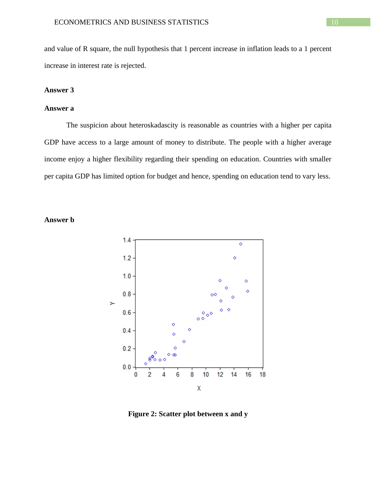
Answer b
Figure 2: Scatter plot between x and y
and value of R square, the null hypothesis that 1 percent increase in inflation leads to a 1 percent
increase in interest rate is rejected.
Answer 3
Answer a
The suspicion about heteroskadascity is reasonable as countries with a higher per capita
GDP have access to a large amount of money to distribute. The people with a higher average
income enjoy a higher flexibility regarding their spending on education. Countries with smaller
per capita GDP has limited option for budget and hence, spending on education tend to vary less.
Answer b
Figure 2: Scatter plot between x and y
11ECONOMETRICS AND BUSINESS STATISTICS
The scatter plot between X and Y reveals that there exists a linear relationship between X and Y.
This indicates presence of heteroskedasticity that is non-constant variance of error terms. In
presence of heteroskadascity, variation in Y differs depending on the variation in X. From the
scatter plot it is seen that small values of X leads to small scatter in Y while large values are
associated with large scatter in Y.
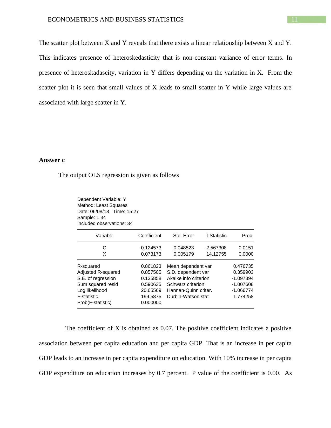
Answer c
The output OLS regression is given as follows
Dependent Variable: Y
Method: Least Squares
Date: 06/08/18 Time: 15:27
Sample: 1 34
Included observations: 34
Variable Coefficient Std. Error t-Statistic Prob.
C -0.124573 0.048523 -2.567308 0.0151
X 0.073173 0.005179 14.12755 0.0000
R-squared 0.861823 Mean dependent var 0.476735
Adjusted R-squared 0.857505 S.D. dependent var 0.359903
S.E. of regression 0.135858 Akaike info criterion -1.097394
Sum squared resid 0.590635 Schwarz criterion -1.007608
Log likelihood 20.65569 Hannan-Quinn criter. -1.066774
F-statistic 199.5875 Durbin-Watson stat 1.774258
Prob(F-statistic) 0.000000
The coefficient of X is obtained as 0.07. The positive coefficient indicates a positive
association between per capita education and per capita GDP. That is an increase in per capita
GDP leads to an increase in per capita expenditure on education. With 10% increase in per capita
GDP expenditure on education increases by 0.7 percent. P value of the coefficient is 0.00. As
The scatter plot between X and Y reveals that there exists a linear relationship between X and Y.
This indicates presence of heteroskedasticity that is non-constant variance of error terms. In
presence of heteroskadascity, variation in Y differs depending on the variation in X. From the
scatter plot it is seen that small values of X leads to small scatter in Y while large values are
associated with large scatter in Y.
Answer c
The output OLS regression is given as follows
Dependent Variable: Y
Method: Least Squares
Date: 06/08/18 Time: 15:27
Sample: 1 34
Included observations: 34
Variable Coefficient Std. Error t-Statistic Prob.
C -0.124573 0.048523 -2.567308 0.0151
X 0.073173 0.005179 14.12755 0.0000
R-squared 0.861823 Mean dependent var 0.476735
Adjusted R-squared 0.857505 S.D. dependent var 0.359903
S.E. of regression 0.135858 Akaike info criterion -1.097394
Sum squared resid 0.590635 Schwarz criterion -1.007608
Log likelihood 20.65569 Hannan-Quinn criter. -1.066774
F-statistic 199.5875 Durbin-Watson stat 1.774258
Prob(F-statistic) 0.000000
The coefficient of X is obtained as 0.07. The positive coefficient indicates a positive
association between per capita education and per capita GDP. That is an increase in per capita
GDP leads to an increase in per capita expenditure on education. With 10% increase in per capita
GDP expenditure on education increases by 0.7 percent. P value of the coefficient is 0.00. As
⊘ This is a preview!⊘
Do you want full access?
Subscribe today to unlock all pages.
Trusted by 1+ million students worldwide
1 out of 15
Related Documents


Your All-in-One AI-Powered Toolkit for Academic Success.
+13062052269
info@desklib.com
Available 24*7 on WhatsApp / Email
![[object Object]](/_next/static/media/star-bottom.7253800d.svg)
Unlock your academic potential
Copyright © 2020–2026 A2Z Services. All Rights Reserved. Developed and managed by ZUCOL.