Econometrics Data Analysis Report

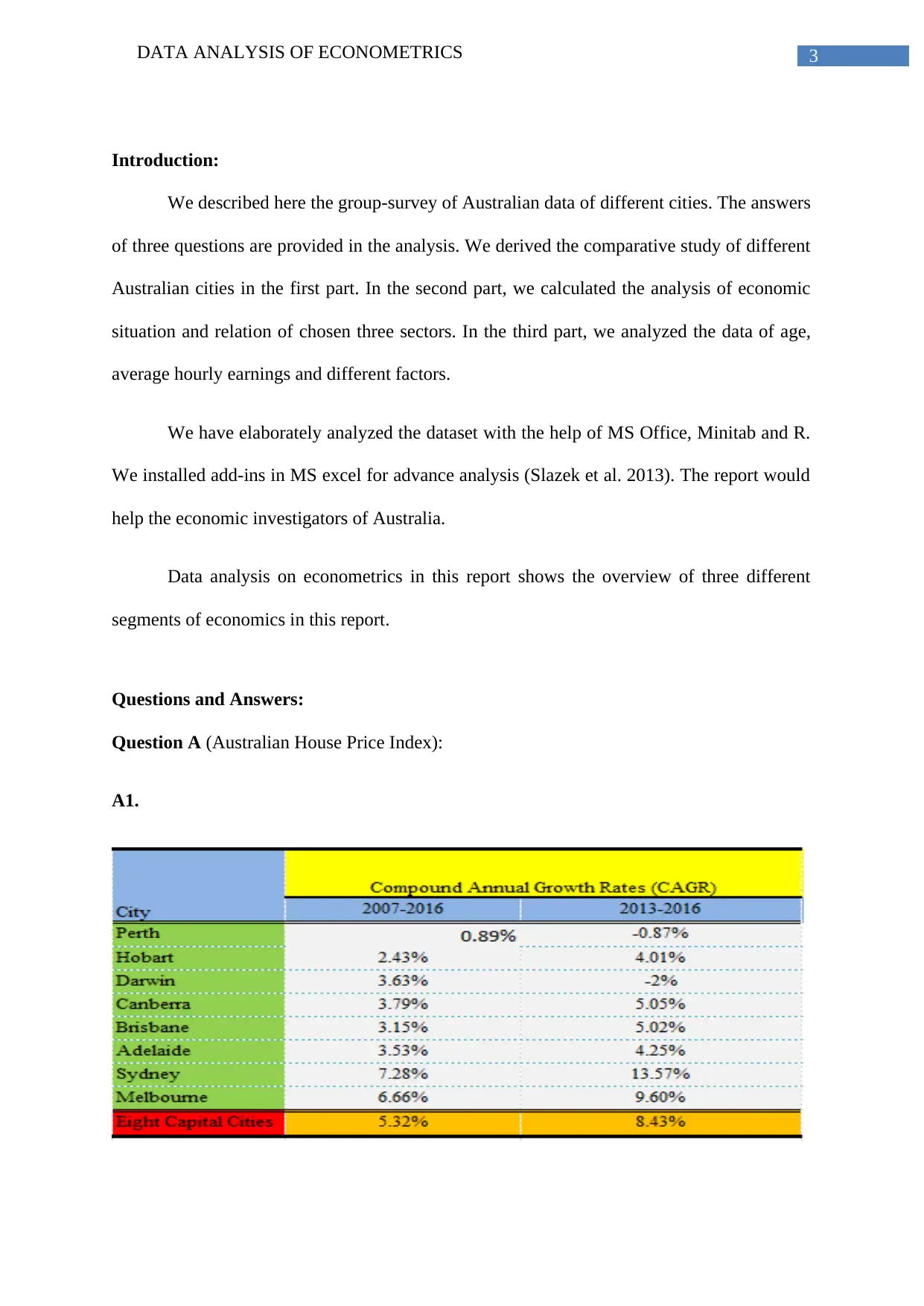
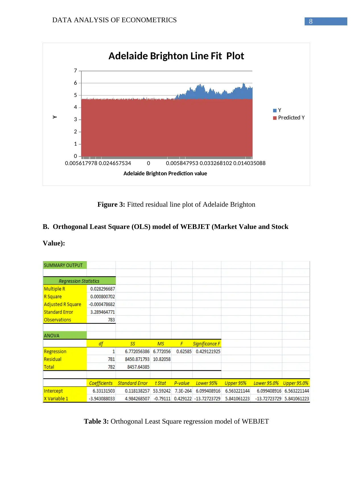
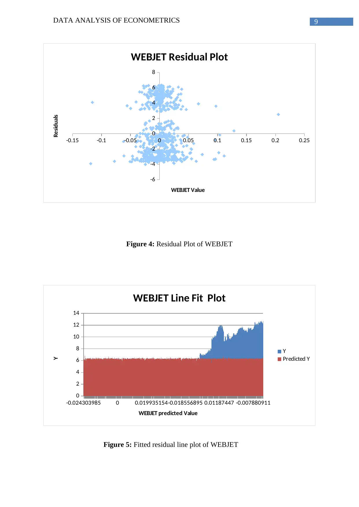
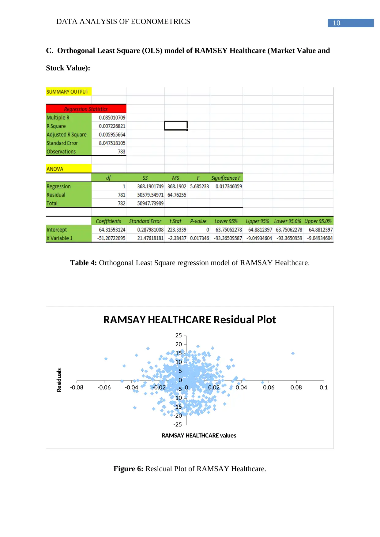
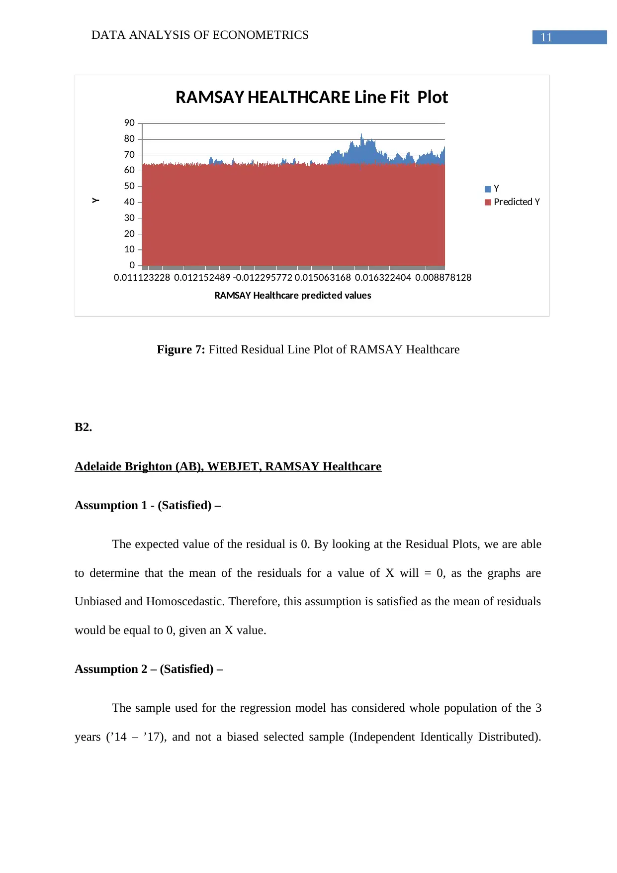
This econometrics report analyzes Australian economic data across three key areas. The first section examines Australian House Price Indices, calculating compound annual growth rates for various cities, mortgage payments, and house price appreciation. The second section uses orthogonal least squares (OLS) regression to model the relationship between market value and stock value for three chosen securities (Adelaide Brighton, Webjet, and Ramsay Healthcare), analyzing betas, R-squared values, and portfolio diversification. The final section investigates the relationship between average hourly earnings (AHE) and factors like age, gender, and education level using multiple regression analysis, testing for statistical significance and omitted variable bias. The report utilizes MS Office, Minitab, and R for data analysis and interpretation, providing detailed calculations, tables, and figures to support its conclusions.

Running head: DATA ANALYSIS OF ECONOMETRICS
Data Analysis of Econometrics
Name of the University:
Name of the Student:
Author’s Note:

DATA ANALYSIS OF ECONOMETRICS 1
Executive Summary:
The report describes economic skills with the help of regression analysis. We answered three
questions and their subparts. We have provided the necessary calculations and tables. We
interpreted from the analysis with the help of MS Office, Minitab and R. We finally have
drawn the conclusions from each question.

DATA ANALYSIS OF ECONOMETRICS 2
Table of Contents
Introduction:...............................................................................................................................3
Questions and Answers:.............................................................................................................3
Question A.............................................................................................................................3
Question B..............................................................................................................................6
Question C............................................................................................................................23
Conclusion:..............................................................................................................................29
Bibliography List:....................................................................................................................30

DATA ANALYSIS OF ECONOMETRICS 3
Introduction:
We described here the group-survey of Australian data of different cities. The answers
of three questions are provided in the analysis. We derived the comparative study of different
Australian cities in the first part. In the second part, we calculated the analysis of economic
situation and relation of chosen three sectors. In the third part, we analyzed the data of age,
average hourly earnings and different factors.
We have elaborately analyzed the dataset with the help of MS Office, Minitab and R.
We installed add-ins in MS excel for advance analysis (Slazek et al. 2013). The report would
help the economic investigators of Australia.
Data analysis on econometrics in this report shows the overview of three different
segments of economics in this report.
Questions and Answers:
Question A (Australian House Price Index):
A1.

DATA ANALYSIS OF ECONOMETRICS 4
Table 1: Compound Annual Growth Rates of Various Australian Cities.
A2.
The city with the lowest growth is Perth at 0.89% in 2007-2016 and the city with the
highest growth is Sydney with 7.28% as shown in the 2013-2016.
A3.
SYDNEY:
The monthly payments are considered as PMT, as the loan is a collection of an annual
interest rate. The periodic payment where in this case the payments are paid monthly.
According to the assignment, the principal amount of Sydney is given as $608768.
To calculate PMT,
PMT = PV * [i / {1 - (1 + i)-n}]
Where, i = 0.5% (compounded monthly from 6%), t = 300 (300 months within 25
years since we are compounded monthly), PV = 608768(675000 – (20% * 675000))
PMT = $608768[0.5% / {1 – (1 + 0.5%)-300}] = $3922.300115
The amount needed to pay back is a total of $3922.3 per month.
A4.

DATA ANALYSIS OF ECONOMETRICS 5
1
3
5
7
9
11
13
15
17
19
21
23
25
27
29
31
33
0%
10%
20%
30%
40%
50%
60%
70%
80%
90%
100%
Principal Amount
Interest Amount of SYDNEY
Figure 1: An Area Diagram shows the comparison between Principal Amount and
Percentage of Interest of Sydney.
The following figures are based off 24th month on data attached
Interest paid = $2937.057583
Principal Paid = $985.2346406
Total = $(2937.05+985.234) = $3922.3 = $3922.3
Percentage of payment paid to principal = 25.12%
A5.
The total amount of interest that will end up paying is = $567922.2263
The figure of total amount of interest is based on the appropriate calculation that also
includes all interest earning.
A6.
In the assignment,

DATA ANALYSIS OF ECONOMETRICS 6
Sydney House Price: $675000
CAGR: 5.05%
Year 25: FV = Current Value*(1+r) n = 675000(1+5.05%) 25 = $2314128.793
House Appreciation = Future Value of House Price – Current Value of House Price
= 2314128.793 – 675000 = $1639128.793
As, $1639128.793 > $567922.2263; Therefore, we can say that, House Appreciation
> Total Interest Paid.
From our above calculation, we can conclude that the value of the house is greater
than the interest paid thus the value appreciation is sufficient to cover the total interest paid.
Question B.
The three chosen securities are industrial in Mix. And Fix., consumer services in
travel and tourism and healthcare providers. The value of ri in the industrial, consumer
services and Healthcare services are calculated separately.
B1.
A. Orthogonal Least Square (OLS) model of Adelaide Brighton (Market Value and
Stock Value):

DATA ANALYSIS OF ECONOMETRICS 7
Table 2: Orthogonal Least Square regression model of Adelaide Brighton
-0.06 -0.04 -0.02 0 0.02 0.04 0.06 0.08 0.1
-2
-1.5
-1
-0.5
0
0.5
1
1.5
Adelaide Brighton Residual Plot
Residuals
Figure 2: Residual Plot of Adelaide Brighton

DATA ANALYSIS OF ECONOMETRICS 8
0.005617978 0.024657534 0 0.005847953 0.033268102 0.014035088
0
1
2
3
4
5
6
7
Adelaide Brighton Line Fit Plot
Y
Predicted Y
Adelaide Brighton Prediction value
Y
Figure 3: Fitted residual line plot of Adelaide Brighton
B. Orthogonal Least Square (OLS) model of WEBJET (Market Value and Stock
Value):
Table 3: Orthogonal Least Square regression model of WEBJET

DATA ANALYSIS OF ECONOMETRICS 9
-0.15 -0.1 -0.05 0 0.05 0.1 0.15 0.2 0.25
-6
-4
-2
0
2
4
6
8
WEBJET Residual Plot
WEBJET Value
Residuals
Figure 4: Residual Plot of WEBJET
-0.024303985 0 0.019935154-0.018556895 0.01187447 -0.007880911
0
2
4
6
8
10
12
14
WEBJET Line Fit Plot
Y
Predicted Y
WEBJET predicted Value
Y
Figure 5: Fitted residual line plot of WEBJET

DATA ANALYSIS OF ECONOMETRICS 10
C. Orthogonal Least Square (OLS) model of RAMSEY Healthcare (Market Value and
Stock Value):
Table 4: Orthogonal Least Square regression model of RAMSAY Healthcare.
-0.08 -0.06 -0.04 -0.02 0 0.02 0.04 0.06 0.08 0.1
-25
-20
-15
-10
-5
0
5
10
15
20
25
RAMSAY HEALTHCARE Residual Plot
RAMSAY HEALTHCARE values
Residuals
Figure 6: Residual Plot of RAMSAY Healthcare.

DATA ANALYSIS OF ECONOMETRICS 11
0.011123228 0.012152489 -0.012295772 0.015063168 0.016322404 0.008878128
0
10
20
30
40
50
60
70
80
90
RAMSAY HEALTHCARE Line Fit Plot
Y
Predicted Y
RAMSAY Healthcare predicted values
Y
Figure 7: Fitted Residual Line Plot of RAMSAY Healthcare
B2.
Adelaide Brighton (AB), WEBJET, RAMSAY Healthcare
Assumption 1 - (Satisfied) –
The expected value of the residual is 0. By looking at the Residual Plots, we are able
to determine that the mean of the residuals for a value of X will = 0, as the graphs are
Unbiased and Homoscedastic. Therefore, this assumption is satisfied as the mean of residuals
would be equal to 0, given an X value.
Assumption 2 – (Satisfied) –
The sample used for the regression model has considered whole population of the 3
years (’14 – ’17), and not a biased selected sample (Independent Identically Distributed).