Econometrics Assignment - Analysis of Earnings and Education Data

Verified

Added on  2023/01/03

|9
|1273
|23
Homework Assignment
AI Summary
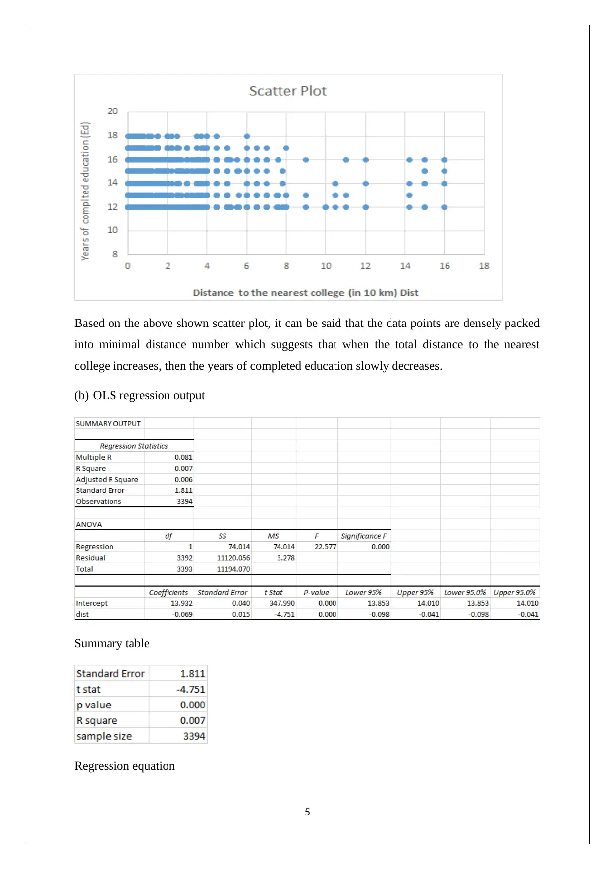
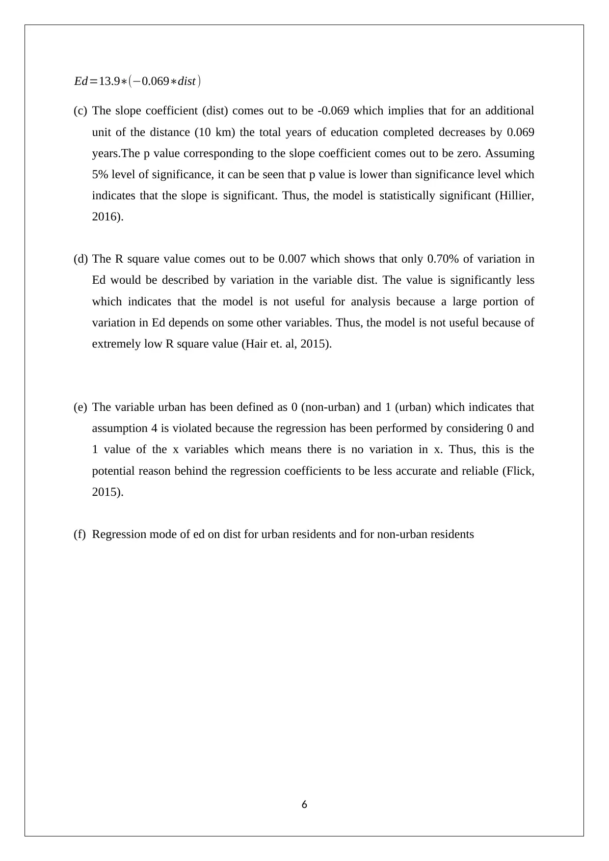
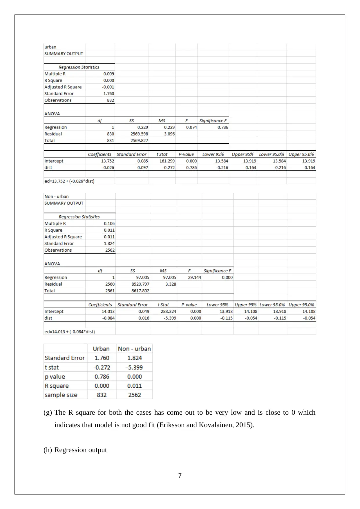
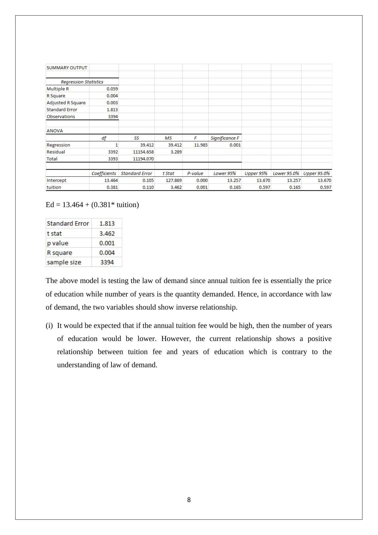
This econometrics assignment solution analyzes a dataset of 5 individuals, examining the relationship between earnings (re78), education (educ), and age. Question 1 involves constructing a frequency table, calculating conditional expectations, sample variance and covariance, and deriving a sample regression line. The solution explores the impact of education on earnings and assesses the statistical significance of the regression coefficients. Question 2 investigates the relationship between distance to college and years of education completed, utilizing OLS regression and analyzing the R-squared value. Further analysis includes the impact of urban vs non-urban residence and tuition fees on education levels, and the application of the law of demand. The solution provides detailed explanations of the statistical concepts and interpretations of the results, including the limitations of the models and the significance of the findings. The assignment concludes with a list of relevant references.
Document Page
ECONOMETRICS
STUDENT ID:
[Pick the date]
tabler-icon-diamond-filled.svg

Paraphrase This Document

Need a fresh take? Get an instant paraphrase of this document with our AI Paraphraser
Document Page
Question 1
(a) Frequency distribution table
Age = < 40 Age > 40
Educ <10 1 2
Educ >= 10 1 1
(b) Relevant table
Answer
E(re78 | educ =11) 11.01
E(re78 | educ>10) = (16.46+11.01)/2 = 13.73
E(re78 | educ<10 and age >30) = (8.35+6.77)/2 = 7.56
E(re78 | educ>8 and age >= 40) = (6.77+16.46)/2 = 11.62
(c) Sample variance of Educ and sample covariance between re78 and Educ
Variance of Educ = VAR () = 4.30
Covariance between re78 and Educ3 = COVAR () = 6.57
(d) Sample regression line
2
Document Page
78=(1.91Educ)8.75
(e) When there is only observation 2 then we will get Error: range error message because
with one observation there would be no variation in x values. Further, the sample size is
lower than the total number of parameters that are estimated. This indicates that this
would cause violation of the 2 assumptions of the CLRM assumption (Flick,2015).
(f) Population model
78=9+2.1 educ +u
Observation re 78 (Y) Educ (X) E(Y/X) u Predicted Y
(Y cap)
Residual
(ucap)
1 8.35 7 5.7 2.65 4.62 3.73
2 6.77 9 9.9 -3.13 8.44 -1.67
3 16.46 12 16.2 0.26 14.17 2.29
4 11.01 11 14.1 -3.09 12.26 -1.25
5 3.44 8 7.8 -4.36 6.53 -3.09
(g) The sum of random errors(u) and the residuals (e) are not the same. This is on expected
lines as the accuracy of the population model would be different in comparison to the
3
Document Page
sample model which has been derived on the basis of the given values only (Hillier,
2016).
(h) The regression equation obtained in part (d) is as follows.
Re78 = -8.75+ 1.91*EDUC
The intercept is -8.75 which represents that if the education of an individual is zero, then the
earnings is negative. Clearly, this is not practical as the lowest earning could be zero. With
regards to the slope coefficient, the positive value suggests that higher years of education
tend to have a positive influence in the income. It is estimated that if the years of education
rises by 1 year, the salary in 1978 would have increased by $ 1,910 per year. The additional
data with regards to p value indicates that the slope coefficient and the intercept both are
statistically insignificant. Assuming a significance level of 5%, both p values are greater than
0.05 which implies that the slope is insignificant. This is also reflected in the form of higher
standard error associated with the regression coefficients (Hair et. al., 2015).
(i) The requisite hypotheses are shown below.
H0: βEDUC = 2.1
Hi: βEDUC ≠2.1
The above test would be a 2 tail test owing to the alternative hypothesis sign.
Further, test statistics (t) = 2.37
Degrees of freedom = 5-2 =3
At 5% significance level, df =3, t critical value = +/- 3.18
It is evident that the test statistic lies in the interval marked by the critical values. Hence, the
available evidence does not warrant rejection of null hypothesis. As a result, it can be
concluded that the regression slope is not significant at 5% significance level (Eriksson and
Kovalainen, 2015).
Question 2
(a) Scatter plot between dist and Ed is shown below.
4
tabler-icon-diamond-filled.svg

Paraphrase This Document

Need a fresh take? Get an instant paraphrase of this document with our AI Paraphraser
Document Page
Based on the above shown scatter plot, it can be said that the data points are densely packed
into minimal distance number which suggests that when the total distance to the nearest
college increases, then the years of completed education slowly decreases.
(b) OLS regression output
Summary table
Regression equation
5
Document Page
Ed=13.9(0.069dist )
(c) The slope coefficient (dist) comes out to be -0.069 which implies that for an additional
unit of the distance (10 km) the total years of education completed decreases by 0.069
years.The p value corresponding to the slope coefficient comes out to be zero. Assuming
5% level of significance, it can be seen that p value is lower than significance level which
indicates that the slope is significant. Thus, the model is statistically significant (Hillier,
2016).
(d) The R square value comes out to be 0.007 which shows that only 0.70% of variation in
Ed would be described by variation in the variable dist. The value is significantly less
which indicates that the model is not useful for analysis because a large portion of
variation in Ed depends on some other variables. Thus, the model is not useful because of
extremely low R square value (Hair et. al, 2015).
(e) The variable urban has been defined as 0 (non-urban) and 1 (urban) which indicates that
assumption 4 is violated because the regression has been performed by considering 0 and
1 value of the x variables which means there is no variation in x. Thus, this is the
potential reason behind the regression coefficients to be less accurate and reliable (Flick,
2015).
(f) Regression mode of ed on dist for urban residents and for non-urban residents
6
Document Page
(g) The R square for both the cases has come out to be very low and is close to 0 which
indicates that model is not good fit (Eriksson and Kovalainen, 2015).
(h) Regression output
7
tabler-icon-diamond-filled.svg

Paraphrase This Document

Need a fresh take? Get an instant paraphrase of this document with our AI Paraphraser
Document Page
Ed = 13.464 + (0.381* tuition)
The above model is testing the law of demand since annual tuition fee is essentially the price
of education while number of years is the quantity demanded. Hence, in accordance with law
of demand, the two variables should show inverse relationship.
(i) It would be expected that if the annual tuition fee would be high, then the number of years
of education would be lower. However, the current relationship shows a positive
relationship between tuition fee and years of education which is contrary to the
understanding of law of demand.
8
Document Page
References
Eriksson, P. and Kovalainen, A. (2015) Quantitative methods in business research. 3rd ed.
London: Sage Publications, pp. 134, 167
Flick, U. (2015) Introducing research methodology: A beginner's guide to doing a research
project. 4th ed. New York: Sage Publications, pp. 156,167
Hair, J. F., Wolfinbarger, M., Money, A. H., Samouel, P., and Page, M. J. (2015) Essentials
of business research methods. 2nd ed. New York: Routledge pp, 178-180
Hillier, F. (2016) Introduction to Operations Research.6th ed.New York: McGraw Hill
Publications, pp. 203-205
9
chevron_up_icon
1 out of 9
circle_padding
hide_on_mobile
zoom_out_icon
[object Object]