Econometrics: Comprehensive Analysis of Linear Regression Techniques

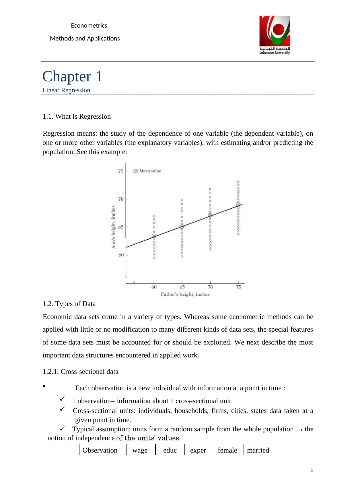
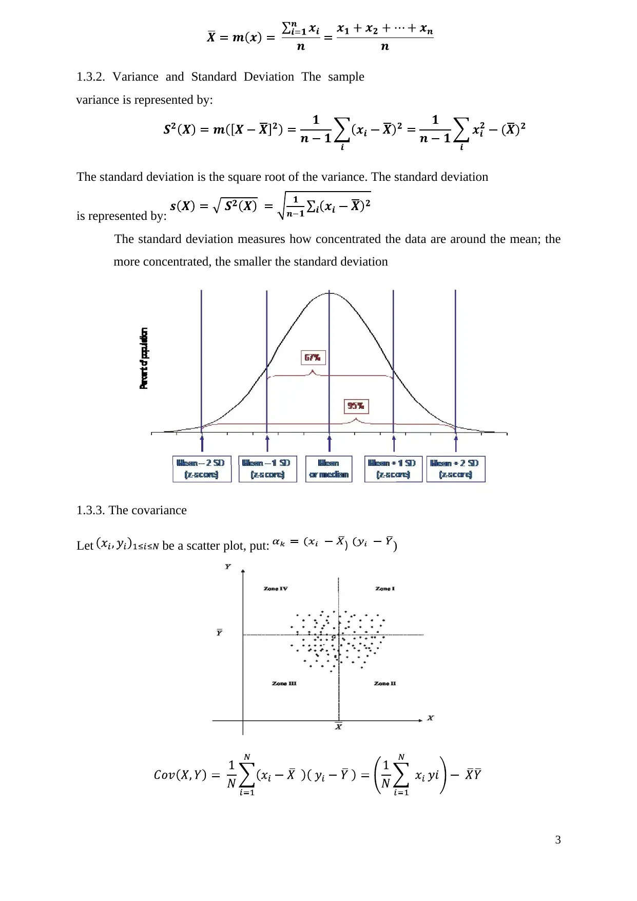
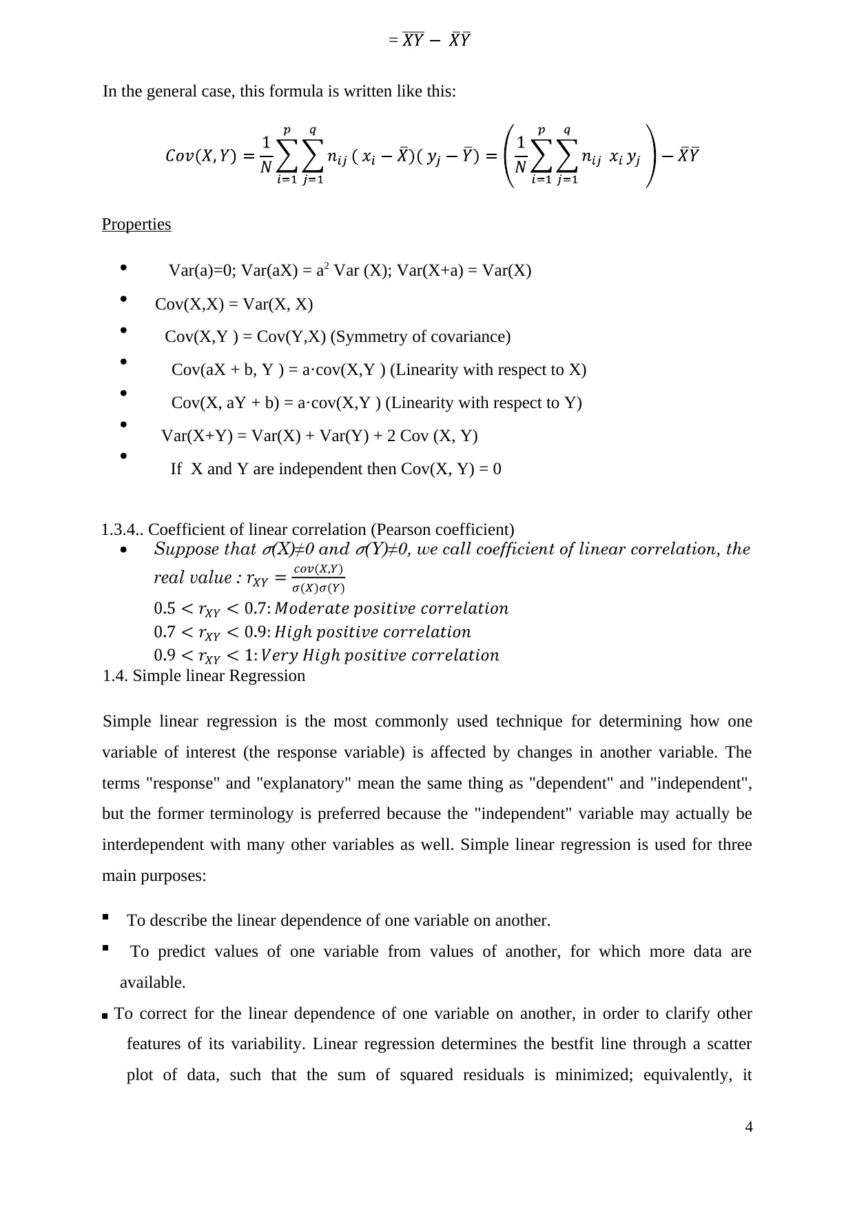
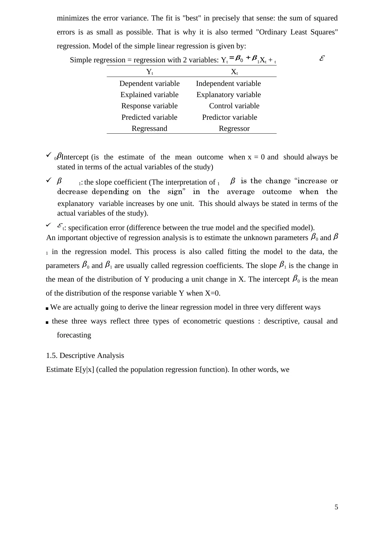
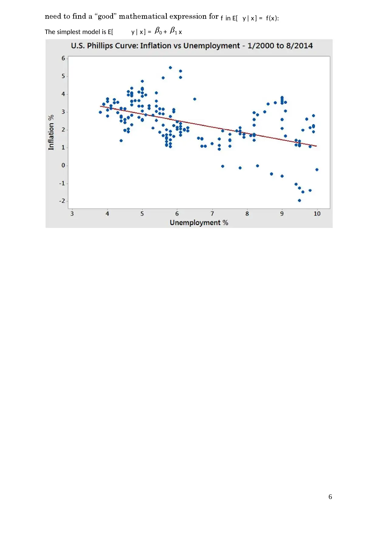
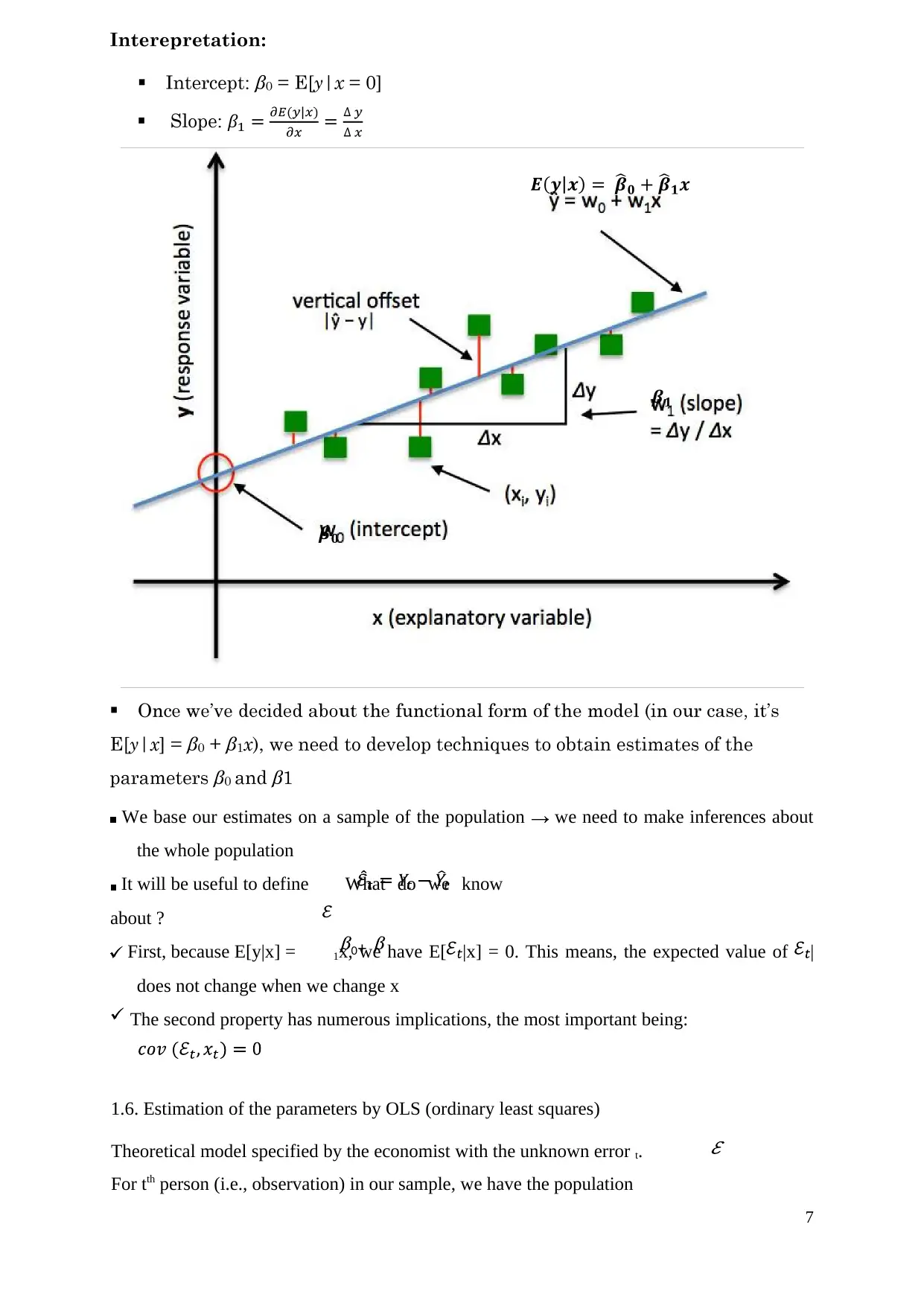
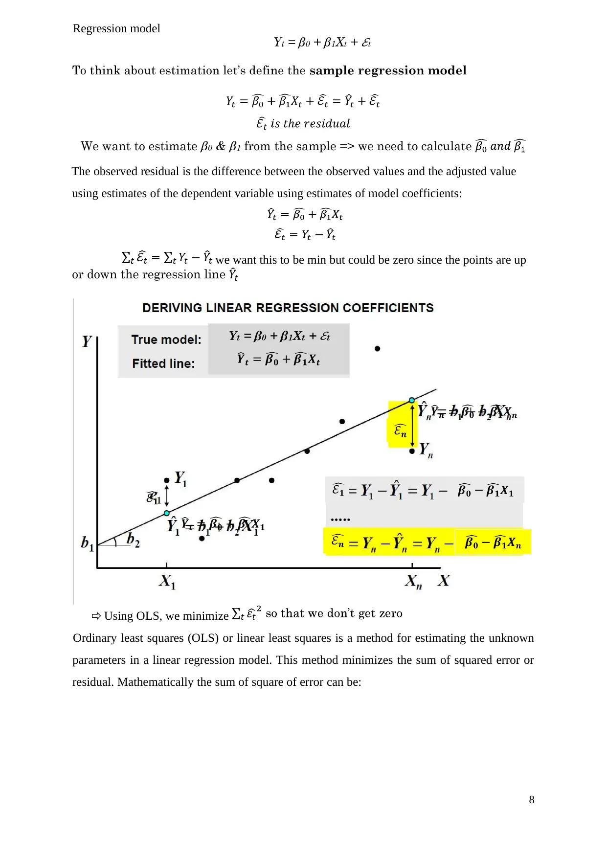
This report provides a comprehensive overview of linear regression within the field of econometrics. It begins by defining regression and its purpose, then explores various data types including cross-sectional, time series, and panel data. Key statistical concepts such as arithmetic mean, variance, covariance, and the coefficient of linear correlation are introduced. The core of the report focuses on simple linear regression, detailing its purposes, the model, and the estimation of parameters using Ordinary Least Squares (OLS). The report explains descriptive analysis and the OLS method, along with the properties of least-square estimators. Furthermore, it connects regression analysis with the analysis of variance and discusses the coefficient of determination, R-squared, and adjusted R-squared. Finally, the report touches upon confidence intervals and significance tests for regression parameters, offering a thorough introduction to linear regression techniques and applications in econometrics.

Chapter 1
Linear Regression
1.1. What is Regression
Regression means: the study of the dependence of one variable (the dependent variable), on
one or more other variables (the explanatory variables), with estimating and/or predicting the
population. See this example:
1.2. Types of Data
Economic data sets come in a variety of types. Whereas some econometric methods can be
applied with little or no modification to many different kinds of data sets, the special features
of some data sets must be accounted for or should be exploited. We next describe the most
important data structures encountered in applied work.
1.2.1. Cross-sectional data
Each observation is a new individual with information at a point in time :
1 observation= information about 1 cross-sectional unit.
Cross-sectional units: individuals, households, firms, cities, states data taken at a
given point in time.
Typical assumption: units form a random sample from the whole population the
notion of independence .
Observation wage educ exper female married
1
Econometrics
Methods and Applications

1 3.10 11 2 1 0
2 3.24 12 22 1 1
525 11.56 16 5 0 0
526 3.5 14 5 1 0
If the data is not a random sample, we have a sample selection problem
1.2.2. Time series data
Observations on economic variables over time
stock prices, money supply, CPI, GDP, annual homicide rates, automobile sales
frequencies: daily, weekly, monthly, quarterly, annually Unlike cross-
sectional data, ordering is important here!
typically, observations cannot be considered independent across time
year T-bill inflation population
2004 4.95 2.6 260,660
2005 5.21 2.8 263,034
1.2.3. Panel (or Longitudinal) data
Panel data or longitudinal data[1][2] are multi-dimensional data involving measurements over
time. Panel data contain observations of multiple phenomena obtained over multiple time
periods for the same individuals
unit year popul murders unemp police
1 2008 293,700 5 6.3 358
1 2010 299,500 7 7.4 396
2 2008 53,450 2 7.2 51
2 2010 51,970 1 8.1 51
1.3. Statistics
1.3.1. Arithmetic Mean
To obtain the value of the arithmetic mean, calculate the sum of the data and divide the result
by the total number of data. X is the symbol of the arithmetic mean.
2

1.3.2. Variance and Standard Deviation The sample
variance is represented by:
The standard deviation is the square root of the variance. The standard deviation
is represented by:
The standard deviation measures how concentrated the data are around the mean; the
more concentrated, the smaller the standard deviation
1.3.3. The covariance
Let be a scatter plot, put: )
3
)

=
In the general case, this formula is written like this:
Properties
Var(a)=0; Var(aX) = a2 Var (X); Var(X+a) = Var(X)
Cov(X,X) = Var(X, X)
Cov(X,Y ) = Cov(Y,X) (Symmetry of covariance)
Cov(aX + b, Y ) = a·cov(X,Y ) (Linearity with respect to X)
Cov(X, aY + b) = a·cov(X,Y ) (Linearity with respect to Y)
Var(X+Y) = Var(X) + Var(Y) + 2 Cov (X, Y)
If X and Y are independent then Cov(X, Y) = 0
1.3.4.. Coefficient of linear correlation (Pearson coefficient)
1.4. Simple linear Regression
Simple linear regression is the most commonly used technique for determining how one
variable of interest (the response variable) is affected by changes in another variable. The
terms "response" and "explanatory" mean the same thing as "dependent" and "independent",
but the former terminology is preferred because the "independent" variable may actually be
interdependent with many other variables as well. Simple linear regression is used for three
main purposes:
To describe the linear dependence of one variable on another.
To predict values of one variable from values of another, for which more data are
available.
To correct for the linear dependence of one variable on another, in order to clarify other
features of its variability. Linear regression determines the bestfit line through a scatter
plot of data, such that the sum of squared residuals is minimized; equivalently, it
4

minimizes the error variance. The fit is "best" in precisely that sense: the sum of squared
errors is as small as possible. That is why it is also termed "Ordinary Least Squares"
regression. Model of the simple linear regression is given by:
Simple regression = regression with 2 variables: Yt 1Xt + t
Yt Xt
Dependent variable Independent variable
Explained variable Explanatory variable
Response variable Control variable
Predicted variable Predictor variable
Regressand Regressor
0: Intercept (is the estimate of the mean outcome when x = 0 and should always be
stated in terms of the actual variables of the study)
1: the slope coefficient (The interpretation of 1
explanatory variable increases by one unit. This should always be stated in terms of the
actual variables of the study).
t: specification error (difference between the true model and the specified model).
An important objective of regression analysis is to estimate the unknown parameters 0 and
1 in the regression model. This process is also called fitting the model to the data, the
parameters 0 and 1 are usually called regression coefficients. The slope 1 is the change in
the mean of the distribution of Y producing a unit change in X. The intercept 0 is the mean
of the distribution of the response variable Y when X=0.
We are actually going to derive the linear regression model in three very different ways
these three ways reflect three types of econometric questions : descriptive, causal and
forecasting
1.5. Descriptive Analysis
Estimate E[y|x] (called the population regression function). In other words, we
5
0

6
f in E[ y| x ] = f(x ):
The simplest model is E[ y| x ] = 0 + 1 x

0+
We base our estimates on a sample of the population we need to make inferences about
the whole population
It will be useful to define What do we know
about ?
First, because E[y|x] = 1x, we have E[ |x] = 0. This means, the expected value of |
does not change when we change x
The second property has numerous implications, the most important being:
1.6. Estimation of the parameters by OLS (ordinary least squares)
Theoretical model specified by the economist with the unknown error t.
For tth person (i.e., observation) in our sample, we have the population
7

Regression model
The observed residual is the difference between the observed values and the adjusted value
using estimates of the dependent variable using estimates of model coefficients:
we want this to be min but could be zero since the points are up
Using OLS, we minimize
Ordinary least squares (OLS) or linear least squares is a method for estimating the unknown
parameters in a linear regression model. This method minimizes the sum of squared error or
residual. Mathematically the sum of square of error can be:
8

Simplifying the above equations we get the following normal equations:
(II)
(III)
are based on a single sample rather than the entire population. If you took different sample,
you would get different values for
the OLS estimators of 0 and 1. One of the main goals of econometrics is to analyze the
quality of these estimators and see under what conditions these are good estimators and under
which conditions they are not.
Properties of Least -Square Estimators:
I. The OLS estimators are expressed solely in terms of the observable (i.e., sample)
quantities (i.e., X and Y). Therefore, they can be easily computed.
II. They are point estimators; that is, given the sample, each estimator will provide only
a single (point) value of the relevant population parameter.
9
and and

III. Once the OLS estimates are obtained from the sample data, the sample regression line
(Figure) can be easily obtained. The regression line thus obtained has the following
properties:
1) It passes through the sample means of Y and X. For the latter can be written as
actual Y for
3) The mean value of the residuals is zero.
4) The residuals are uncorrelated with Xt
Remark:
These properties are contained in the well-known Gauss Markov theorem. To understand this
theorem, we need to consider the best linear unbiasedness property of an estimator. As
explained above, an estimator, say the OLS
estimator , is said to be a best linear unbiased estimator (OLS estimator is
systematically overestimate/underestimate the true
parameters 1 if the following hold:
1. It is linear, that is, a linear function of a random variable, such as the dependent
variable Y in the regression model.
2. It is unbiased, that is, its average or expected value, E( ), is equal to the true
10
, which is shown diagrammatically in Figure below
2) The mean value of the estimated Y = is equal to the mean value of the

value, 1 : E( ) 1
and
So
3. It has minimum variance in the class of all such linear unbiased estimators; an
unbiased estimator with the least variance is known as an efficient estimator.
(Best Linear Unbiased Estimator)
Example 1: Relationship between wage and eduction. wage =
average hourly earnings educ = years of education
Data is collected in 1976, n = 526
...
Figure: Scatter plot of the data with regression line.
11

Model Estimation results :
additional year increases hourly wage on average by 0.54 dollars.
1.7. Regression Analysis and Analysis Of Variance
In this section we study regression analysis from the point of view of the analysis of variance
and introduce the reader to an illuminating and complementary way of looking at the
statistical inference problem.
Instead of using a test based on the distribution of the OLS estimator, we could test the
significance of the slope by comparing the simple linear regression model with the null
model. Note that these models are nested, because we can obtain the null model by setting =
0 in the simple linear regression model.
The sum squares of the residuals, often called the error sum of squares is:
SSE =
The sum squares of the regressions is:
SSR =
The sum squares of the total is:
SST =
12
...
The estimated model is: -0.905 + 0.541 x . Thus the model predicts that an
=

SST = SSR + SSE
This equation will allow us to judge the quality of the fit of a model. Over the explained
variance (SSR) is close to the total variance (SST), better the fit of the cloud point to the
simple linear regression.
1.8. The coefficient of Determination:
1.8.1. The goodness of fit coefficient: R-Square
- The coefficient of determination, R2, is useful because it gives the proportion of the
variance of one variable that is predictable from the other variable.
- The coefficient of determination is the ratio of the explained variation to the total variation
-
strength of the linear association between X and Y.
- R2 = 1 only if SSE = 0, which means that all residuals are zero, and all observations lie
exactly on the regression line
- R2 = 0 only if SSR = 0, which implies that
- The coefficient of determination represents the percent of the data that is the closest to the
line of best fit. For example, if r = 0.922, then r2 = 0.850, which means that 85% of the
total variation in y can be explained by the linear relationship between X and Y. The other
15% of the total variation in y remains unexplained.
13
2

Remark: Coefficient of linear correlation:
1.8.2.3. Adjusted R-square:
where k = number of independent variables.
The adjusted R2 can be used for comparing two models.
1.9. Confidence intervals and significance tests for regression parameters
1.9.1 Confidence intervals CIs for regression parameters
Under the assumptions that the observation are normally and independently distributed and t
~ Normal (0, ).
Confidence intervals CIs for 1
(k = 1 in simple regression)
We use the t distribution, now with n 2 degrees of freedom. A level CI confidence interval
Where is is the appropriate value from the t table (student table)
Confidence intervals CIs for 0
14
Before we do inference for the slope parameter 1, we need the standard variance
for the estimate 1 ( 1) and the residual variance :
for the slope, 1, is:
Before we do inference for the slope parameter 0, we need the variance for the
estimate 0 ( 0) and the residual variance .

We use the t distribution, now with n 2 degrees of freedom. A level CI confidence interval at
the critical value
1.9.2. Testing the Significance of Regression Coefficients (Test for individual significance)
An alternative but complementary approach to the confidence-interval method of testing
statistical hypotheses is the test-of-significance approach developed along independent lines
by R. A. Fisher and jointly by Neyman and Pearson. Broadly speaking, a test of significance
is a procedure by which sample results are used to verify the truth or falsity of a null
hypothesis. The key idea behind tests of significance is that of a test statistic (estimator) and
the sampling distribution of such a statistic under the null hypothesis. The decision to accept
or reject H0 is made on the basis of the value of the test statistic obtained from the data at
hand. As an illustration, recall that under the normality assumption the variable.
If there is a significant linear relationship between the independent variable X and the
dependent variable Y, the slope will not equal zero
Hypothesis Step1:
15
for the slope, 1, is:
0
0.02
0.04
0.06
0.08
0.1
0.12
1 2 3 5 6 7 8 9 10
Mean 12 13 14 15 16 17 18 19 20 21
Region of Non
rejection of H0
Critical Value Critical Value
Rejection
RegionRejection
Region

H0: i = 0 (use y y to predict y, there is no linear relationship between x and y)
H1: i 0 (use to predict Y, there is a stat sig linear relationship between X and
Y)
The null hypothesis states that the slope is equal to zero, and the alternative hypothesis states
that the slope is not equal to zero
Formulate an Analysis Plan
The analysis plan describes how to use sample data to accept or reject the null hypothesis.
The plan should specify the following elements.
Significance level. Often, researchers choose significance levels (critical value) equal to
0.01, 0.05, or 0.10; but any value between 0 and 1 can be used.
Test method. Use a linear regression t-test (Student test) to determine whether the slope of
the regression line differs significantly from zero.
Step 2:
This is a two-tailed test [two-sided]. It is based on the statistical Student t-test calculated as
follows:
Step 3: Critical value from student table Step
4: Decision rule:
1.9.10. F-test of Overall Significance in Regression Analysis
In general, an F-test in regression compares the fits of different linear models. Unlike t-tests
that can assess only one regression coefficient at a time, the F-test can assess multiple
coefficients simultaneously.
16

The F-test of the overall significance is a specific form of the F-test. It compares a model with
no predictors to the model that you specify. A regression model that contains no predictors is
also known as an intercept-only model.
The hypotheses for the F-test of the overall significance are as follows:
Null hypothesis: i = 0
Alternative hypothesis: otherwise
ANOVA Table for Simple Linear Regression
Source degree of
freedom (df)
Sum of Squares Mean Squares F value p-value
Model k ( yi y )2 = SSR Due
to Regression = MSR
Pr(F > F(k, n k-1))
Residual n k-1 2
i = SSE
Due to residual = MSE
Total n 1 (yi y )2= SSTotal
MST
Remark: In the case of simple linear regression, the F test is identical to test individual
significance of the slope. Both tests are based on the same
assumptions, and is demonstrated in this case that:
Decision rule:
1.9.3. Prediction of new observation:
An important application of regression model is predicting new or future observation Y
corresponding to a specified level of the regression variable X.
Prediction interval on a future observation Y0 at the value Xh is given by at
17
1 2

1.10. Assumptions of linear regression
When you choose to analyze your data using linear regression, part of the process involves
checking to make sure that the data you want to analyze can actually be analyzed using linear
regression. You need to do this because it is only appropriate to use linear regression if your
data "passes" six assumptions that are required for linear regression to give you a valid result.
In practice, checking for these assumptions just adds a little bit more time to your analysis,
requiring you to click a few more buttons in SPSS Statistics when performing your analysis,
as well as think a little bit more about your data, but it is not a difficult task.
Before we introduce you to these six assumptions, do not be surprised if, when analysing your
own data using SPSS Statistics, one or more of these assumptions is violated (i.e., not met).
This is not uncommon when working with real-world data rather than textbook examples,
which often only show you how to carry out
your data fails certain assumptions, there is often a solution to overcome this.
Assumption 1: There needs to be a linear relationship between the two variables. Whilst
there are a number of ways to check whether a linear relationship exists between your two
variables, we suggest creating a scatterplot using SPSS Statistics where you can plot the
dependent variable against your independent variable and then visually inspect the scatter-
plot to check for linearity. Your scatter-plot may look something like one of the
following:
If the relationship displayed in your scatter-plot is not linear, you will have to either run a
non-linear regression analysis, perform a polynomial regression or "transform" your data,
which you can do using SPSS Statistics. In our enhanced guides, we show you how to: (a)
create a scatter-plot to check for linearity when carrying out linear regression using SPSS
18

Statistics; (b) interpret different scatter-plot results; and (c) transform your data using SPSS
Statistics if there is not a linear relationship between your two variables.
Assumption 2: You should have independence of observations, which you can easily check
using the Durbin-Watson statistic, which is a simple test to run using SPSS Statistics. We
explain how to interpret the result of the Durbin-Watson statistic in our enhanced linear
regression guide.
Assumption 3: Your data needs to show homoscedasticity, which is where the variances
along the line of best fit remain similar as you move along the line. Whilst we explain
more about what this means and how to assess the homoscedasticity of your data in our
enhanced linear regression guide, take a look at the three scatter-plots below, which
provide three simple examples: two of data that fail the assumption (called
heteroscedasticity) and one of data that meets this assumption (called homoscedasticity):
Whilst these help to illustrate the differences in data that meets or violates the assumption of
homoscedasticity, real-world data can be a lot more messy and illustrate different patterns of
heteroscedasticity. Therefore, in our enhanced linear regression guide, we explain: (a) some of
the things you will need to consider when interpreting your data; and (b) possible ways to
continue with your analysis if your data fails to meet this assumption.
Assumption 4: statistical independence of the errors (no autocorrelation between the
disturbances)
An error at time t does not affect the following errors
19

Assumption 5: You need to check that the residuals (errors) of the regression line are
approximately normally distributed (we explain these terms in our enhanced linear
regression guide). Two common methods to check this assumption include using either a
histogram (with a superimposed normal curve) or a Normal Q-Q Plot. Again, in our
enhanced linear regression guide, we: (a) show you how to check this assumption using
SPSS Statistics, whether you use a histogram (with superimposed normal curve) or
Normal QQ Plot; (b) explain how to interpret these diagrams; and (c) provide a possible
solution if your data fails to meet this assumption. t 2).
Assumption 6: There is no exact linear relationship (i.e. Multicolinearity) in the repressors.
1.11. The term of linear
Linearity in the variables: Our previous example, Y is linear expression of X, but
1 2X2 is not.
Linearity in the parameters.
The conditional expectation of Y (E(Y|X)) is a linear function of the parameters.
20
o What about 1 2X 2 this time?
o How about 1 + X ?

1.12. Changing units of measurement (Non linearity)
Nonlinear models can be classified into two categories.
In the first category are models that are nonlinear in the variables, but still linear in terms of
the unknown parameters. This category includes models which are made linear in the
parameters via a transformation.
For example, the Cobb-Douglas production function that relates output (Y) to
la
bor (L) and capital (K) can be written as: the least squares technique.
1.12.1. Double log Model (Log-Log) and Elasticity
The double log model is the most common functional form. Although it is nonlinear in the
variables it is linear in coefficients.
In a double log functional form the natural log of Y is the dependent variable and the natural
log ln of the X(s) are the independent variable.
This model is frequently used because it has constant, elasticity whilst the slopes are not.
In the double log model, measures the elasticity=
Example: Cobb-Douglas Production function The log-
lin model :
The lin-log
model:
The second category of nonlinear models contains models which are nonlinear in the
parameters and which cannot be made linear in the parameters after a transformation.
For estimating models in this category the familiar least squares technique is extended to an
estimation procedure known as nonlinear least squares.
Example: E[ log(wage) | educ ] = 0 + 1 educ
21
:

This is still considered to be a linear regression model; the word linear actually means
linear in parameters
Remark: Log-transformation can be only applied to variables that assume strictly positive
values!
22
Logarithm transform is one of the basic econometric tools
the rule to remember: taking the log of one of the variables means we shift
from absolute changes to relative changes: