Econometrics Assignment: Regression Analysis and Statistical Inference
VerifiedAdded on 2021/12/08
|28
|4390
|481
Homework Assignment
AI Summary
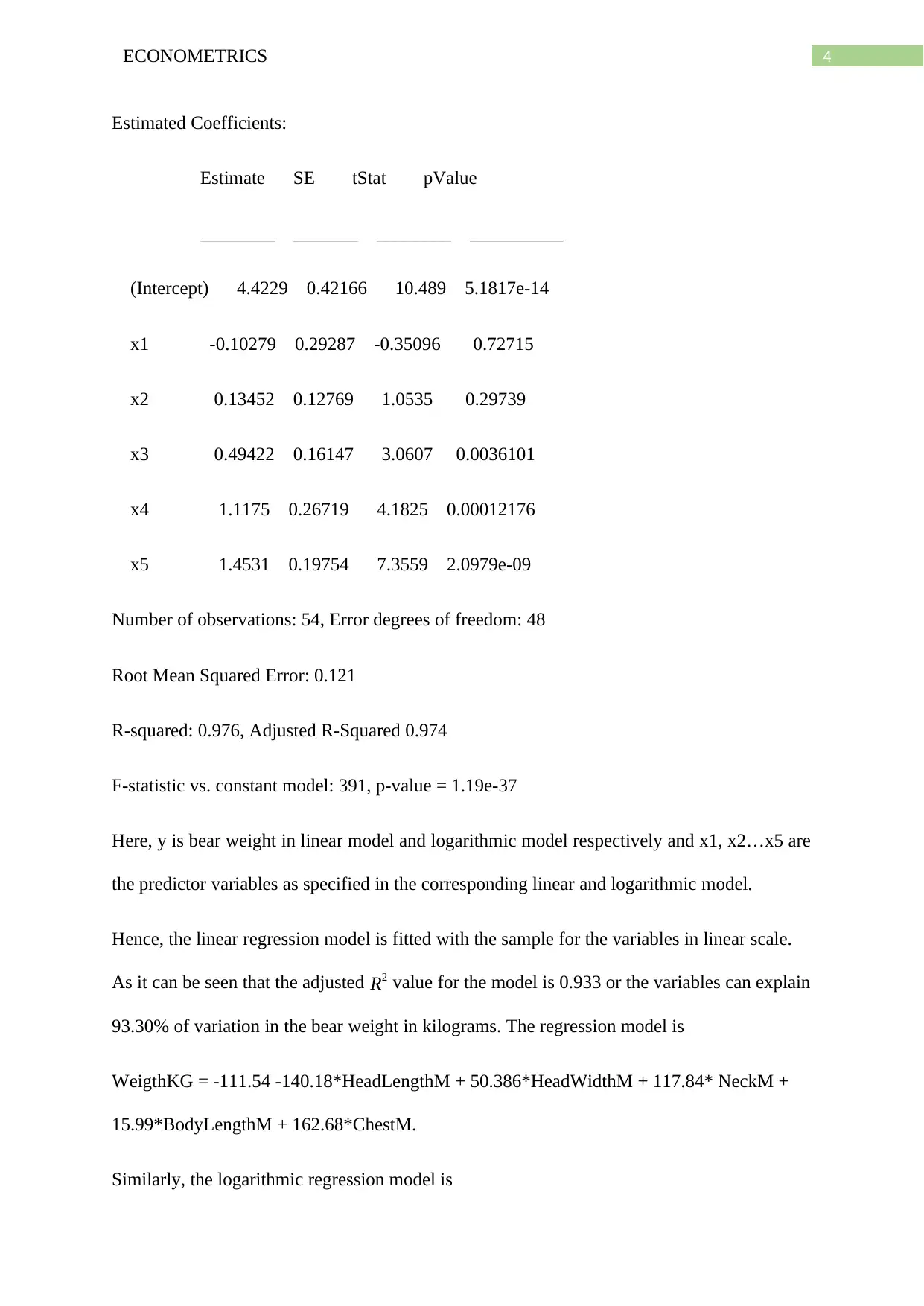
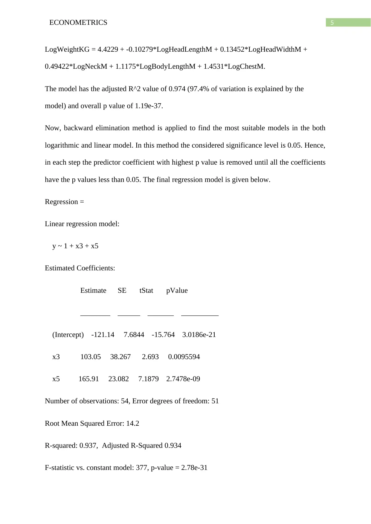
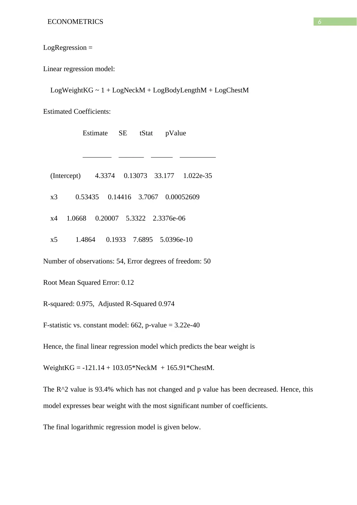
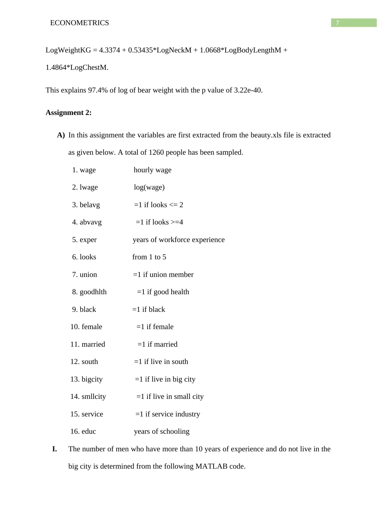
This econometrics assignment presents three distinct problems. The first involves predicting bear weight using linear and logarithmic regression models, analyzing variables like head length, neck circumference, and chest circumference, and applying backward elimination to refine the models. The second problem focuses on wage analysis, exploring the relationship between hourly wage and variables such as experience, education, and looks, using linear regression and coefficient tests. The third part generates independent and identically distributed random variables, calculates their correlation, and visualizes the data through a scatter plot, demonstrating the concept of independence and probability. The assignment utilizes MATLAB for data manipulation, model fitting, and statistical analysis, providing detailed outputs and interpretations of the results.

Running head: ECONOMETRICS
ECONOMETRICS
Name of the Student
Name of the University
Author Note
ECONOMETRICS
Name of the Student
Name of the University
Author Note
Paraphrase This Document
Need a fresh take? Get an instant paraphrase of this document with our AI Paraphraser

1ECONOMETRICS
Assignment 1:
In this assignment all the variables from the ‘bears.xls’ files are first extracted and then a
prediction model(regression) for bear weight is performed with respect to other variables
chosen as independent variables. The variables are listed as follows.
MonthObs: The month in which each of bears are measured.
Gender: The gender of bears, 1 = male and 2 =female
HeadLengthInches: Head length of the bears measured in inches.
NeckInches: Circumference of the neck of bears measured in inches.
BodyLengthInches: length of the body of bears measured in inches.
ChestInches: circumference of the chest of bears measured in inches.
WeightPounds: Weight of the bears measured in pounds.
The sample of 54 bears is collected by the scientist assumed are collected in random
sampling method. From the sample the regression is performed to measure the weight of the
bears as it is practically very much difficult or impossible to measure the weight of the bears
individually. The linear regression model is performed in MATLAB which is shown below.
All the units are converted to metric form (weight of bears in Kgs and lengths or
circumference in meters).
MATLAB code:
bears = readtable('bears.xls','ReadVariableNames',true);
Meter = 1*0.0254; % inch to meter conversion unit
KGs = 1*0.45359227; % pounds to Kg conversion unit

2ECONOMETRICS
HeadLengthM = bears.HeadLengthInches.*Meter;
HeadWidthM = bears.HeadWidthInches.*Meter;
NeckM = bears.NeckInches.*Meter;
BodyLengthM = bears.BodyLengthInches.*Meter;
ChestM = bears.ChestInches.*Meter;
WeightKG = bears.WeightPounds.*KGs;
Regression = fitlm([HeadLengthM HeadWidthM NeckM BodyLengthM
ChestM],WeightKG) % Regression with linear variables
LogHeadLengthM = log(HeadLengthM);
LogHeadWidthM = log(HeadWidthM);
LogNeckM = log(NeckM);
LogBodyLengthM = log(BodyLengthM);
LogChestM = log(ChestM);
LogWeightKG = log(WeightKG);
LogRegression = fitlm([LogHeadLengthM LogHeadWidthM LogNeckM
LogBodyLengthM LogChestM],LogWeightKG) % Fitting Regression with logarithmic
variables
Output:
assign1
Regression =
⊘ This is a preview!⊘
Do you want full access?
Subscribe today to unlock all pages.

Trusted by 1+ million students worldwide

3ECONOMETRICS
Linear regression model:
y ~ 1 + x1 + x2 + x3 + x4 + x5
Estimated Coefficients:
Estimate SE tStat pValue
________ ______ _______ __________
(Intercept) -111.54 14.393 -7.7493 5.2791e-10
x1 -140.18 103.78 -1.3508 0.18309
x2 50.386 89.738 0.56148 0.57708
x3 117.84 45.874 2.5687 0.013373
x4 15.99 21.178 0.75504 0.45391
x5 162.68 26.201 6.2089 1.2017e-07
Number of observations: 54, Error degrees of freedom: 48
Root Mean Squared Error: 14.3
R-squared: 0.939, Adjusted R-Squared 0.933
F-statistic vs. constant model: 148, p-value = 5.57e-28
LogRegression =
Linear regression model:
y ~ 1 + x1 + x2 + x3 + x4 + x5
Linear regression model:
y ~ 1 + x1 + x2 + x3 + x4 + x5
Estimated Coefficients:
Estimate SE tStat pValue
________ ______ _______ __________
(Intercept) -111.54 14.393 -7.7493 5.2791e-10
x1 -140.18 103.78 -1.3508 0.18309
x2 50.386 89.738 0.56148 0.57708
x3 117.84 45.874 2.5687 0.013373
x4 15.99 21.178 0.75504 0.45391
x5 162.68 26.201 6.2089 1.2017e-07
Number of observations: 54, Error degrees of freedom: 48
Root Mean Squared Error: 14.3
R-squared: 0.939, Adjusted R-Squared 0.933
F-statistic vs. constant model: 148, p-value = 5.57e-28
LogRegression =
Linear regression model:
y ~ 1 + x1 + x2 + x3 + x4 + x5
Paraphrase This Document
Need a fresh take? Get an instant paraphrase of this document with our AI Paraphraser

4ECONOMETRICS
Estimated Coefficients:
Estimate SE tStat pValue
________ _______ ________ __________
(Intercept) 4.4229 0.42166 10.489 5.1817e-14
x1 -0.10279 0.29287 -0.35096 0.72715
x2 0.13452 0.12769 1.0535 0.29739
x3 0.49422 0.16147 3.0607 0.0036101
x4 1.1175 0.26719 4.1825 0.00012176
x5 1.4531 0.19754 7.3559 2.0979e-09
Number of observations: 54, Error degrees of freedom: 48
Root Mean Squared Error: 0.121
R-squared: 0.976, Adjusted R-Squared 0.974
F-statistic vs. constant model: 391, p-value = 1.19e-37
Here, y is bear weight in linear model and logarithmic model respectively and x1, x2…x5 are
the predictor variables as specified in the corresponding linear and logarithmic model.
Hence, the linear regression model is fitted with the sample for the variables in linear scale.
As it can be seen that the adjusted R2 value for the model is 0.933 or the variables can explain
93.30% of variation in the bear weight in kilograms. The regression model is
WeigthKG = -111.54 -140.18*HeadLengthM + 50.386*HeadWidthM + 117.84* NeckM +
15.99*BodyLengthM + 162.68*ChestM.
Similarly, the logarithmic regression model is

5ECONOMETRICS
LogWeightKG = 4.4229 + -0.10279*LogHeadLengthM + 0.13452*LogHeadWidthM +
0.49422*LogNeckM + 1.1175*LogBodyLengthM + 1.4531*LogChestM.
The model has the adjusted R^2 value of 0.974 (97.4% of variation is explained by the
model) and overall p value of 1.19e-37.
Now, backward elimination method is applied to find the most suitable models in the both
logarithmic and linear model. In this method the considered significance level is 0.05. Hence,
in each step the predictor coefficient with highest p value is removed until all the coefficients
have the p values less than 0.05. The final regression model is given below.
Regression =
Linear regression model:
y ~ 1 + x3 + x5
Estimated Coefficients:
Estimate SE tStat pValue
________ ______ _______ __________
(Intercept) -121.14 7.6844 -15.764 3.0186e-21
x3 103.05 38.267 2.693 0.0095594
x5 165.91 23.082 7.1879 2.7478e-09
Number of observations: 54, Error degrees of freedom: 51
Root Mean Squared Error: 14.2
R-squared: 0.937, Adjusted R-Squared 0.934
F-statistic vs. constant model: 377, p-value = 2.78e-31
⊘ This is a preview!⊘
Do you want full access?
Subscribe today to unlock all pages.

Trusted by 1+ million students worldwide

6ECONOMETRICS
LogRegression =
Linear regression model:
LogWeightKG ~ 1 + LogNeckM + LogBodyLengthM + LogChestM
Estimated Coefficients:
Estimate SE tStat pValue
________ _______ ______ __________
(Intercept) 4.3374 0.13073 33.177 1.022e-35
x3 0.53435 0.14416 3.7067 0.00052609
x4 1.0668 0.20007 5.3322 2.3376e-06
x5 1.4864 0.1933 7.6895 5.0396e-10
Number of observations: 54, Error degrees of freedom: 50
Root Mean Squared Error: 0.12
R-squared: 0.975, Adjusted R-Squared 0.974
F-statistic vs. constant model: 662, p-value = 3.22e-40
Hence, the final linear regression model which predicts the bear weight is
WeightKG = -121.14 + 103.05*NeckM + 165.91*ChestM.
The R^2 value is 93.4% which has not changed and p value has been decreased. Hence, this
model expresses bear weight with the most significant number of coefficients.
The final logarithmic regression model is given below.
Paraphrase This Document
Need a fresh take? Get an instant paraphrase of this document with our AI Paraphraser

7ECONOMETRICS
LogWeightKG = 4.3374 + 0.53435*LogNeckM + 1.0668*LogBodyLengthM +
1.4864*LogChestM.
This explains 97.4% of log of bear weight with the p value of 3.22e-40.
Assignment 2:
A) In this assignment the variables are first extracted from the beauty.xls file is extracted
as given below. A total of 1260 people has been sampled.
1. wage hourly wage
2. lwage log(wage)
3. belavg =1 if looks <= 2
4. abvavg =1 if looks >=4
5. exper years of workforce experience
6. looks from 1 to 5
7. union =1 if union member
8. goodhlth =1 if good health
9. black =1 if black
10. female =1 if female
11. married =1 if married
12. south =1 if live in south
13. bigcity =1 if live in big city
14. smllcity =1 if live in small city
15. service =1 if service industry
16. educ years of schooling
I. The number of men who have more than 10 years of experience and do not live in the
big city is determined from the following MATLAB code.

8ECONOMETRICS
MATLAB code:
%(A)
beauty = readtable('beauty.xls','ReadVariableNames',true);
beauty.Properties.VariableNames = {'wage' 'lwage' 'belavg' 'abvavg' 'exper' 'looks'
'union' 'goodhlth' 'black' 'female' 'married' 'south' 'bigcity' 'smllcity' 'service' 'educ'};
%(I)
men_more10_smallcity = beauty.female == 0 & beauty.exper >= 10 &
beauty.bigcity == 0;
num_men_more10_smllcity = sum(men_more10_smallcity)
Output:
num_men_more10_smllcity =
487
Hence, 487 men are more than 10 years of experience and do not live in big city or
live in small city.
II. The married men who are good health and who live in big city are calculated by the
following code.
MATLAB code:
beauty = readtable('beauty.xls','ReadVariableNames',true);
beauty.Properties.VariableNames = {'wage' 'lwage' 'belavg' 'abvavg' 'exper' 'looks'
'union' 'goodhlth' 'black' 'female' 'married' 'south' 'bigcity' 'smllcity' 'service' 'educ'};
%(II)
menmarriedandgood = beauty.female == 0 & beauty.married == 1 &
beauty.goodhlth==1 & beauty.bigcity == 1;
nummenmarriedandgood = sum(menmarriedandgood)
Output:
MATLAB code:
%(A)
beauty = readtable('beauty.xls','ReadVariableNames',true);
beauty.Properties.VariableNames = {'wage' 'lwage' 'belavg' 'abvavg' 'exper' 'looks'
'union' 'goodhlth' 'black' 'female' 'married' 'south' 'bigcity' 'smllcity' 'service' 'educ'};
%(I)
men_more10_smallcity = beauty.female == 0 & beauty.exper >= 10 &
beauty.bigcity == 0;
num_men_more10_smllcity = sum(men_more10_smallcity)
Output:
num_men_more10_smllcity =
487
Hence, 487 men are more than 10 years of experience and do not live in big city or
live in small city.
II. The married men who are good health and who live in big city are calculated by the
following code.
MATLAB code:
beauty = readtable('beauty.xls','ReadVariableNames',true);
beauty.Properties.VariableNames = {'wage' 'lwage' 'belavg' 'abvavg' 'exper' 'looks'
'union' 'goodhlth' 'black' 'female' 'married' 'south' 'bigcity' 'smllcity' 'service' 'educ'};
%(II)
menmarriedandgood = beauty.female == 0 & beauty.married == 1 &
beauty.goodhlth==1 & beauty.bigcity == 1;
nummenmarriedandgood = sum(menmarriedandgood)
Output:
⊘ This is a preview!⊘
Do you want full access?
Subscribe today to unlock all pages.

Trusted by 1+ million students worldwide

9ECONOMETRICS
nummenmarriedandgood =
133
Hence, there are 133 men who are in good health and live in big city.
B)
I) Now, the linear regression model of log(wage) is fitted with MATLAB in this
part.
The natural log of hourly wage is fitted by regression line with respect to the other
independent variables as given below.
The regression model is given by,
lwage = β0 + β1*exper + β2*exper^2 + β3*educ + μ
Hence, the MATLAB function of fitlm for implementing this model will be
fitlm(beauty,'lwage ~ exper + exper^2 + educ')
Now, when the coefficients β1 and β2 are non-linear function of educ then the
modified regression will be of the form
lwage = β0 + (α0 + α1*educ)*exper + (α2 + α3)*exper^2 + β3*educ + μ
Hence, the MATLAB function of fitlm for implementing the model will be
fitlm(beauty,'lwage ~ exper + educ*exper + exper^2 + educ*exper^2 + educ')
Now, the coefficient test of the regression coefficients can be obtained by the coefTest
function in MATLAB, This determines the p value of the coefficient.
MATLAB code:
beauty = readtable('beauty.xls','ReadVariableNames',true);
beauty.Properties.VariableNames = {'wage' 'lwage' 'belavg' 'abvavg' 'exper' 'looks'
'union' 'goodhlth' 'black' 'female' 'married' 'south' 'bigcity' 'smllcity' 'service' 'educ'};
%(B)
beauty.educXexper = (beauty.educ.*beauty.exper);
Paraphrase This Document
Need a fresh take? Get an instant paraphrase of this document with our AI Paraphraser

10ECONOMETRICS
beauty.eeduc = (beauty.educ);
beauty.educXexper2 = (beauty.educ.*beauty.exper.^2);
normalREG = fitlm(beauty,'lwage ~ exper + exper^2 + educ')
modifiedRegression = fitlm(beauty,'lwage ~ exper + educ*exper + exper^2 +
educ*exper^2 + educ')
CoeficientTestexpsqr = coefTest(modifiedRegression,[0 0 0 1 0 0])
CoeficientTesteduc = coefTest(modifiedRegression,[0 0 0 0 0 1])
CoeficientTestexpsqrandeduc = coefTest(modifiedRegression,[0 0 0 1 0 1])
Output:
normalREG =
Linear regression model:
lwage ~ 1 + exper + educ + exper^2
Estimated Coefficients:
Estimate SE tStat pValue
___________ __________ _______ __________
(Intercept) 0.22669 0.08384 2.7039 0.006946
exper 0.047972 0.0047955 10.004 1.0152e-22
educ 0.070588 0.0057811 12.21 1.7578e-32
exper^2 -0.00069106 0.00010797 -6.4004 2.1842e-10
Number of observations: 1259, Error degrees of freedom: 1255
Root Mean Squared Error: 0.523
R-squared: 0.228, Adjusted R-Squared 0.226
F-statistic vs. constant model: 123, p-value = 6.03e-70
modifiedRegression =

11ECONOMETRICS
Linear regression model:
lwage ~ 1 + exper*educ + exper^2 + (exper^2):educ
Estimated Coefficients:
Estimate SE tStat pValue
___________ __________ _______ ________
(Intercept) 0.53352 0.24651 2.1643 0.03063
exper 0.0081129 0.02438 0.33276 0.73937
educ 0.045287 0.019566 2.3146 0.020798
exper:educ 0.0033031 0.0019588 1.6863 0.091981
exper^2 0.0002062 0.00050714 0.40658 0.68438
exper^2:educ -7.5159e-05 4.1263e-05 -1.8214 0.068777
Number of observations: 1259, Error degrees of freedom: 1253
Root Mean Squared Error: 0.523
R-squared: 0.23, Adjusted R-Squared 0.227
F-statistic vs. constant model: 74.7, p-value = 1.36e-68
CoeficientTestexpsqr =
0.0920
CoeficientTesteduc =
0.0688
CoeficientTestexpsqrandeduc =
0.0928
II) Hence, the modified regression model is
⊘ This is a preview!⊘
Do you want full access?
Subscribe today to unlock all pages.

Trusted by 1+ million students worldwide
1 out of 28
Related Documents

Your All-in-One AI-Powered Toolkit for Academic Success.
+13062052269
info@desklib.com
Available 24*7 on WhatsApp / Email
Unlock your academic potential
Copyright © 2020–2025 A2Z Services. All Rights Reserved. Developed and managed by ZUCOL.