Econometrics Report: R-squared Interpretation and Regression Models

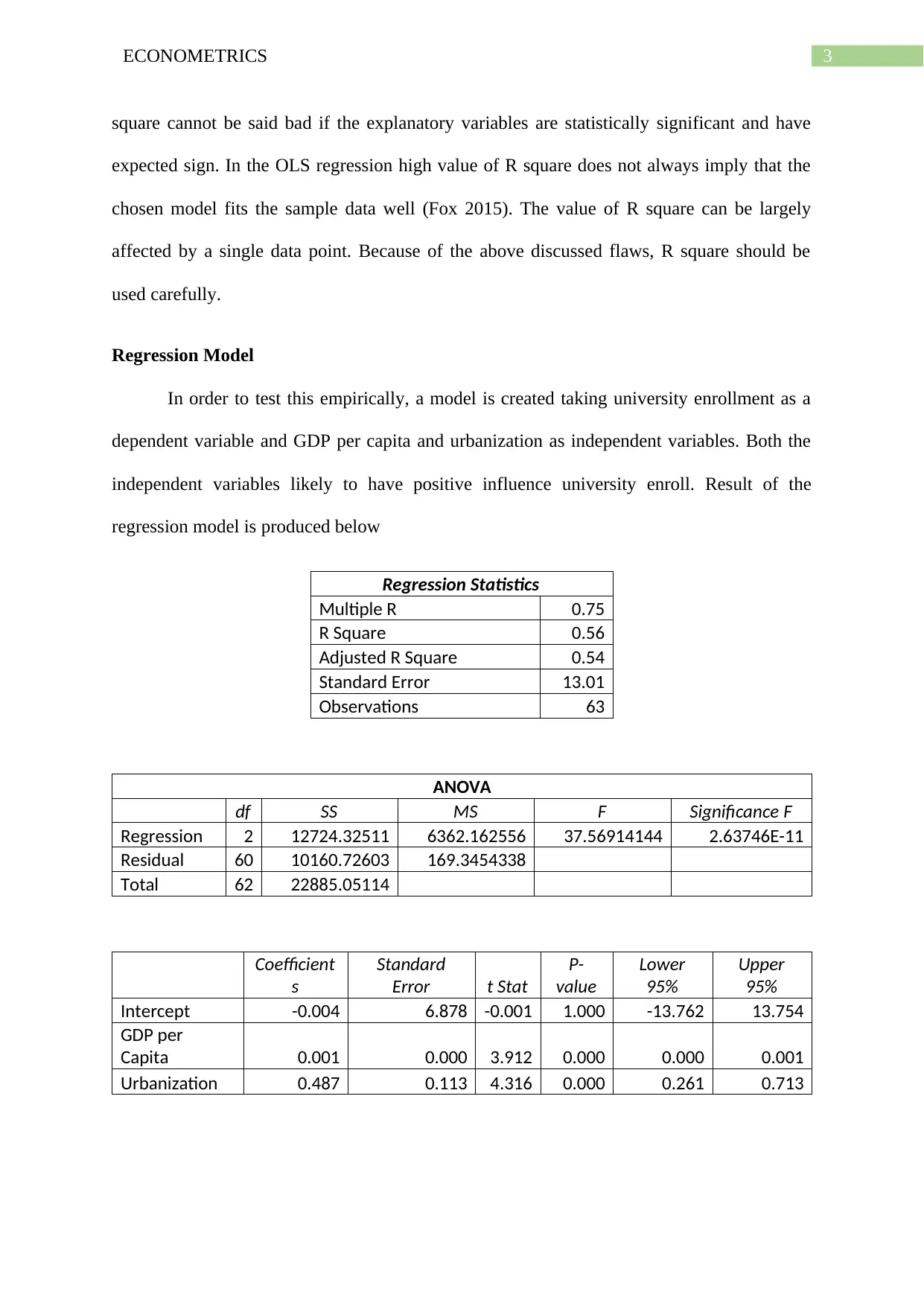
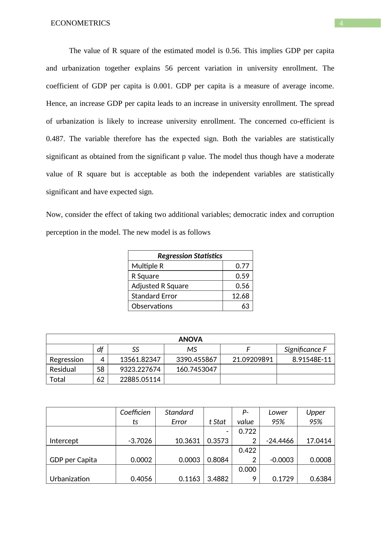
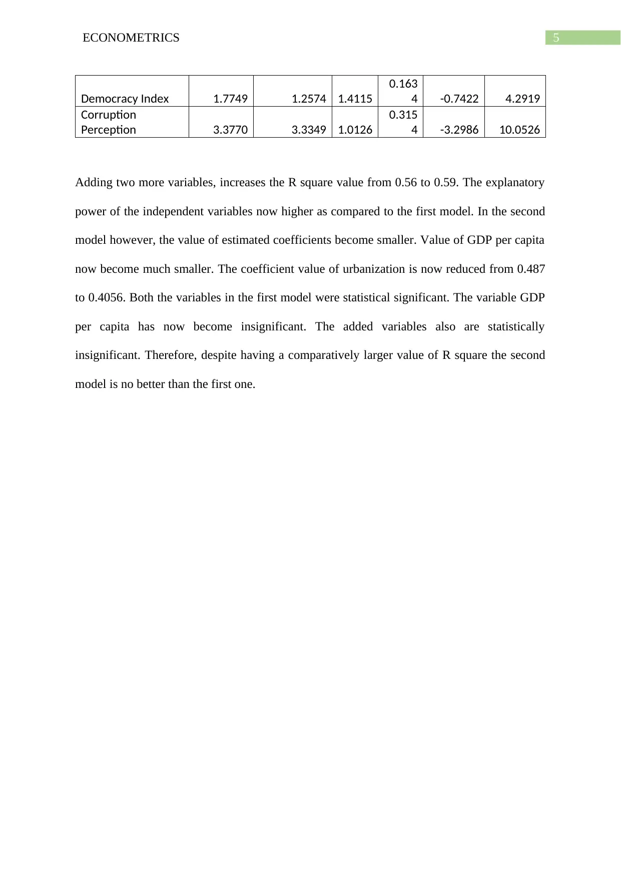
This report provides an analysis of R-squared statistics and their application in econometrics, emphasizing the importance of careful interpretation and avoiding misuse. It discusses how researchers often attempt to maximize R-squared values by adding independent variables, which can lead to models with high R-squared but low statistical significance. The report includes a regression model using university enrollment as the dependent variable and GDP per capita and urbanization as independent variables, demonstrating the impact of adding democratic index and corruption perception variables. It concludes that a model with a moderate R-squared but statistically significant and theoretically relevant variables is preferable to a model with a high R-squared but insignificant variables. Desklib offers a range of past papers and solved assignments for students seeking further assistance.

Running Head: ECONOMETRICS
Econometrics
Name of the Student
Name of the University
Author note

1ECONOMETRICS
Table of Contents
Careful handling of R square.....................................................................................................2
Regression Model.......................................................................................................................3
References..................................................................................................................................6

2ECONOMETRICS
Careful handling of R square
R-square statistics offers a useful measure for the goodness of fit of a linear or
multiple regression model. The R square statistics is also helpful to understand the relevance
or explanatory power of the chosen explanatory variables of the estimated model. The value
of R square lies between 0 and 1. A value closer to 1 implies the chosen explanatory variables
cannot explain much variation of the dependent variables and hence, the estimated model is
considered to be a bad fit (Wooldridge 2008) In other words, the explanatory variables are
not much relevant for the concerned variables. On the other hand, an R square value close to
1, implies the explanatory variables are able to explain much variation and hence the
estimated model is a good fit model.
Despite the usefulness of R square as a measure of goodness of fit, researchers should
be cautious regarding the possible misuse of R square statistics. As high value of R square is
an indication towards a good fit model, researchers always tries to get a high value of R
square. It is however dangerous to play the game of maximizing R square value (Wang, Jiang
and Liu 2017). Some researchers often try to manipulate R square value and increase R
square value as much as possible. Researchers attempts to maximize the value of R square by
gradually increasing the number of independent variables. R square is an increasing function
of number of explanatory variables. In the empirical research, there often arrive a situation in
which the value of R square is very high but very few explanatory variables have statistical
significance or have expected signs (Draper and Smith 2014). Therefore, the model only with
a high R square value is not accepted.
Researchers should give more attention to the theoretical or logical relevance of the
explanatory variables and their statistical significance. In the process, if a high value of R
square is obtained then this is well and good. In contrast a model with a low value of R

3ECONOMETRICS
square cannot be said bad if the explanatory variables are statistically significant and have
expected sign. In the OLS regression high value of R square does not always imply that the
chosen model fits the sample data well (Fox 2015). The value of R square can be largely
affected by a single data point. Because of the above discussed flaws, R square should be
used carefully.
Regression Model
In order to test this empirically, a model is created taking university enrollment as a
dependent variable and GDP per capita and urbanization as independent variables. Both the
independent variables likely to have positive influence university enroll. Result of the
regression model is produced below
Regression Statistics
Multiple R 0.75
R Square 0.56
Adjusted R Square 0.54
Standard Error 13.01
Observations 63
ANOVA
df SS MS F Significance F
Regression 2 12724.32511 6362.162556 37.56914144 2.63746E-11
Residual 60 10160.72603 169.3454338
Total 62 22885.05114
Coefficient
s
Standard
Error t Stat
P-
value
Lower
95%
Upper
95%
Intercept -0.004 6.878 -0.001 1.000 -13.762 13.754
GDP per
Capita 0.001 0.000 3.912 0.000 0.000 0.001
Urbanization 0.487 0.113 4.316 0.000 0.261 0.713

4ECONOMETRICS
The value of R square of the estimated model is 0.56. This implies GDP per capita
and urbanization together explains 56 percent variation in university enrollment. The
coefficient of GDP per capita is 0.001. GDP per capita is a measure of average income.
Hence, an increase GDP per capita leads to an increase in university enrollment. The spread
of urbanization is likely to increase university enrollment. The concerned co-efficient is
0.487. The variable therefore has the expected sign. Both the variables are statistically
significant as obtained from the significant p value. The model thus though have a moderate
value of R square but is acceptable as both the independent variables are statistically
significant and have expected sign.
Now, consider the effect of taking two additional variables; democratic index and corruption
perception in the model. The new model is as follows
Regression Statistics
Multiple R 0.77
R Square 0.59
Adjusted R Square 0.56
Standard Error 12.68
Observations 63
ANOVA
df SS MS F Significance F
Regression 4 13561.82347 3390.455867 21.09209891 8.91548E-11
Residual 58 9323.227674 160.7453047
Total 62 22885.05114
Coefficien
ts
Standard
Error t Stat
P-
value
Lower
95%
Upper
95%
Intercept -3.7026 10.3631
-
0.3573
0.722
2 -24.4466 17.0414
GDP per Capita 0.0002 0.0003 0.8084
0.422
2 -0.0003 0.0008
Urbanization 0.4056 0.1163 3.4882
0.000
9 0.1729 0.6384

5ECONOMETRICS
Democracy Index 1.7749 1.2574 1.4115
0.163
4 -0.7422 4.2919
Corruption
Perception 3.3770 3.3349 1.0126
0.315
4 -3.2986 10.0526
Adding two more variables, increases the R square value from 0.56 to 0.59. The explanatory
power of the independent variables now higher as compared to the first model. In the second
model however, the value of estimated coefficients become smaller. Value of GDP per capita
now become much smaller. The coefficient value of urbanization is now reduced from 0.487
to 0.4056. Both the variables in the first model were statistical significant. The variable GDP
per capita has now become insignificant. The added variables also are statistically
insignificant. Therefore, despite having a comparatively larger value of R square the second
model is no better than the first one.

6ECONOMETRICS
References
Draper, N.R. and Smith, H., 2014. Applied regression analysis(Vol. 326). John Wiley &
Sons.
Fox, J., 2015. Applied regression analysis and generalized linear models. Sage Publications.
Wang, X., Jiang, B. and Liu, J.S., 2017. Generalized R-squared for detecting
dependence. Biometrika, 104(1), pp.129-139.
Wooldridge, J., 2008. Introductory Econometrics: A Modern Approach (with Economic
Applications, Data Sets, Student Solutions Manual Printed Access Card). South-Western
College Pub, 4, p.29.