Econometrics Assignment: Analysis of Economic Data and Models
VerifiedAdded on 2020/10/05
|16
|2449
|55
Homework Assignment
AI Summary
This econometrics assignment focuses on analyzing consumption expenditure using both simple and multiple regression models. The student utilizes hypothetical data and Excel to perform ordinary least squares (OLS) estimations, generate scatter diagrams illustrating relationships between variables like income and wealth, and conduct t-tests and F-tests at a 5% significance level. The assignment covers the interpretation of regression coefficients, the coefficient of determination, and the evaluation of hypotheses. The student explores the relationship between consumption expenditure and annual disposable income and level of wealth, providing interpretations of the regression results and conducting statistical tests to assess the significance of the findings. The analysis includes predicting total consumer expenditure using the generated regression equations and evaluating the overall results. The solution includes the use of Excel for calculations and statistical tests.
ECONOMETRIC
Paraphrase This Document
Need a fresh take? Get an instant paraphrase of this document with our AI Paraphraser
Table of Contents
QUESTION......................................................................................................................................3
Hypothetical Data: Parts A and B..........................................................................................3
Part (A): Simple Linear Regression Model............................................................................3
(1)(b) Scatter diagram depicting Relationship between Total Consumption Expenditure and
Level of Wealth:.....................................................................................................................4
2.(a) Estimation and Interpretation of Regression by Ordinary Least Squares Method using
Excel:......................................................................................................................................5
2.(b) T-test conducted at 5% significance level.....................................................................5
3.(a)Determination of coefficient of determination and generating F-test output..................5
4.(a)Estimation and Interpretation of Regression by Ordinary Least Squares Method.........6
4.(b) T-test conducted at 5% significance level using Excel:................................................6
5.(a)generating F-test output using information in regression summary...............................7
6.Predicting total consumer expenditure using sample regression equation..........................7
Part (B): Multiple Regression Model:..............................................................................................8
7.Linear Regression Data under Multiple Regression Model................................................8
9.Calculation of Coefficient of multiple determination.........................................................8
10. Testing null hypotheses at 5% significance level.............................................................9
11.Testing joint hypotheses at 5% significance level...........................................................10
12: Findings..........................................................................................................................10
13: Evaluation of the results.................................................................................................10
APPENDIX:...................................................................................................................................12
QUESTION
Hypothetical Data: Parts A and B
The table shown in Appendix provides data consisting of a dependent variable (Y), Total
consumption expenditure on non-durables and services and two independent variables, Annual
Disposable Income and Level of Wealth.
Part (A): Simple Linear Regression Model
Simple Linear Regression Model explains the relationship between two or more
variables, of which one is a dependent variable and other is independent variable. Independent
variables are denoted by letter X and dependent variables are denoted by letter Y. The relation
between these two can be explained with the help of the equation Y=a+bx+c where, Y is the
dependent variable; a is the intercept term; b denotes regression coefficient on independent
variable; x denotes independent variable and e denotes residual error. In order to draw
conclusions easily, researchers usually take help of graphs such as Scatter diagrams.
Scatter Diagrams:
Scatter Diagrams are graphical representation of two variables that show any correlation
between the variables. Generally, the first variable represents an independent variable (X) and a
dependent variable (Y), Total Consumption Expenditure in this case. The above sample takes
two independent variables for the value of X- Annual disposable income and Level of wealth.
The scatter diagrams depicting the relationship between these independent variables and
independent variables has been shown below:
(a) Scatter diagram depicting relationship between Total Consumption Expenditure and Annual
Disposable Income:
⊘ This is a preview!⊘
Do you want full access?
Subscribe today to unlock all pages.
Trusted by 1+ million students worldwide
0 200 400 600 800 1000 1200
0
100
200
300
400
500
600
700
800
900
1000
Annual Disposable Income
Total Consumption Expenditure
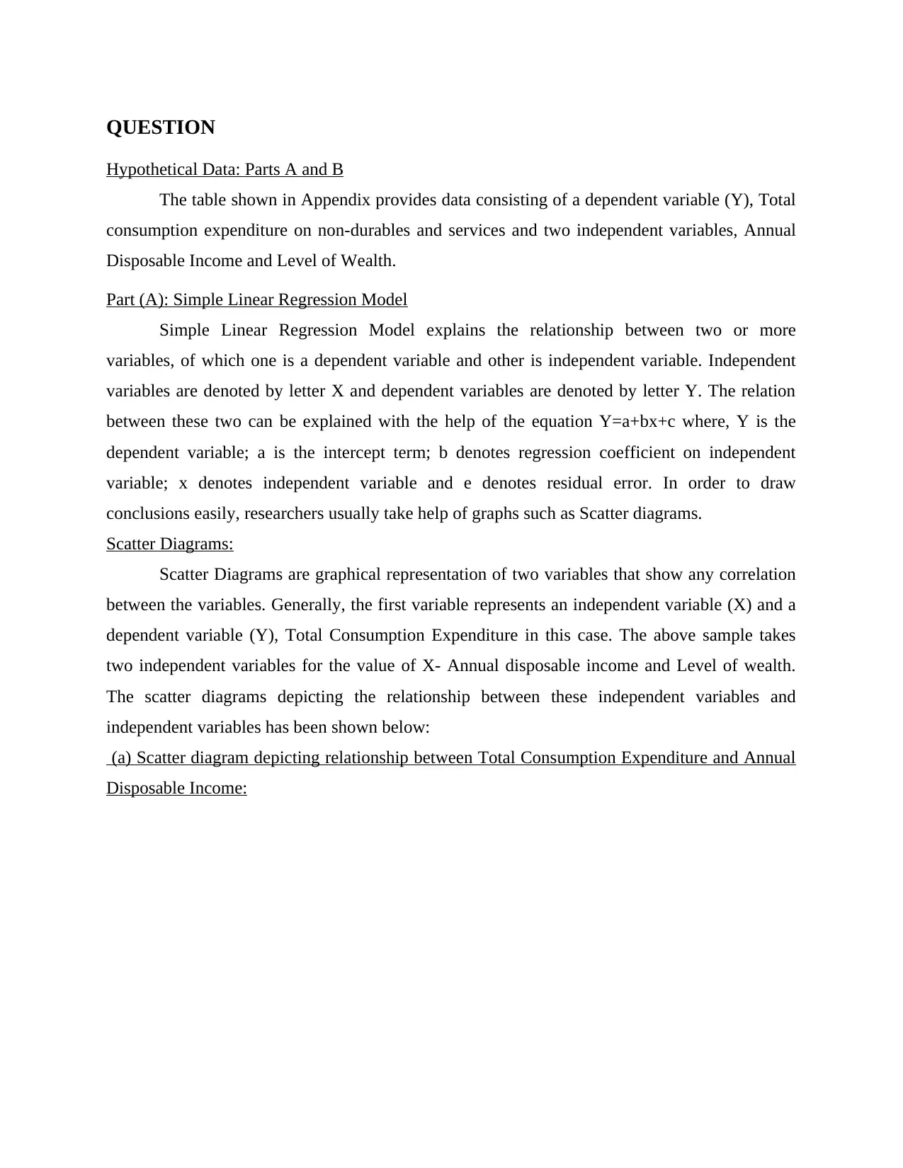
Interpretation: The X-axis plots Annual Disposable Income (independent variable) and
Y-axis plots Total Consumption Expenditure (dependent variable). The scatter diagram shows a
positive correlation among the two variables as they are not scattered very far away from each
other. This straight line is called Linear Regression Line. It is clear from the scatter plot that as
the annual disposable income of an individual increases the correlation between the consumption
expenditure and income gets weaker although remaining positive.
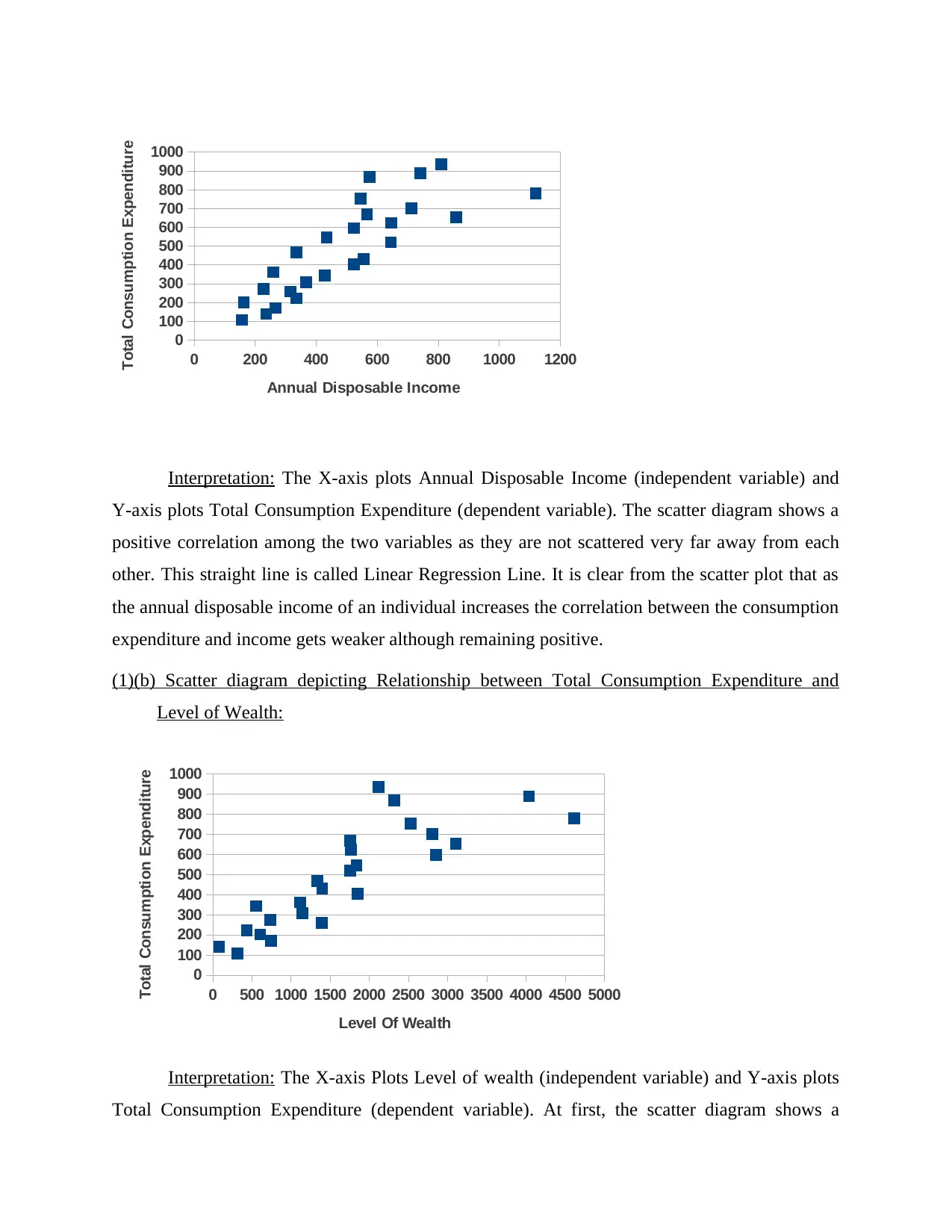
(1)(b) Scatter diagram depicting Relationship between Total Consumption Expenditure and
Level of Wealth:
0 500 1000 1500 2000 2500 3000 3500 4000 4500 5000
0
100
200
300
400
500
600
700
800
900
1000
Level Of Wealth
Total Consumption Expenditure
Interpretation: The X-axis Plots Level of wealth (independent variable) and Y-axis plots
Total Consumption Expenditure (dependent variable). At first, the scatter diagram shows a
0
100
200
300
400
500
600
700
800
900
1000
Annual Disposable Income
Total Consumption Expenditure
Interpretation: The X-axis plots Annual Disposable Income (independent variable) and
Y-axis plots Total Consumption Expenditure (dependent variable). The scatter diagram shows a
positive correlation among the two variables as they are not scattered very far away from each
other. This straight line is called Linear Regression Line. It is clear from the scatter plot that as
the annual disposable income of an individual increases the correlation between the consumption
expenditure and income gets weaker although remaining positive.
(1)(b) Scatter diagram depicting Relationship between Total Consumption Expenditure and
Level of Wealth:
0 500 1000 1500 2000 2500 3000 3500 4000 4500 5000
0
100
200
300
400
500
600
700
800
900
1000
Level Of Wealth
Total Consumption Expenditure
Interpretation: The X-axis Plots Level of wealth (independent variable) and Y-axis plots
Total Consumption Expenditure (dependent variable). At first, the scatter diagram shows a
Paraphrase This Document
Need a fresh take? Get an instant paraphrase of this document with our AI Paraphraser
strong positive correlation among the two variables as they are plotted very closely to each other.
However, as the level of wealth increases the correlation between the consumption expenditure
and wealth gets weaker although remaining positive.
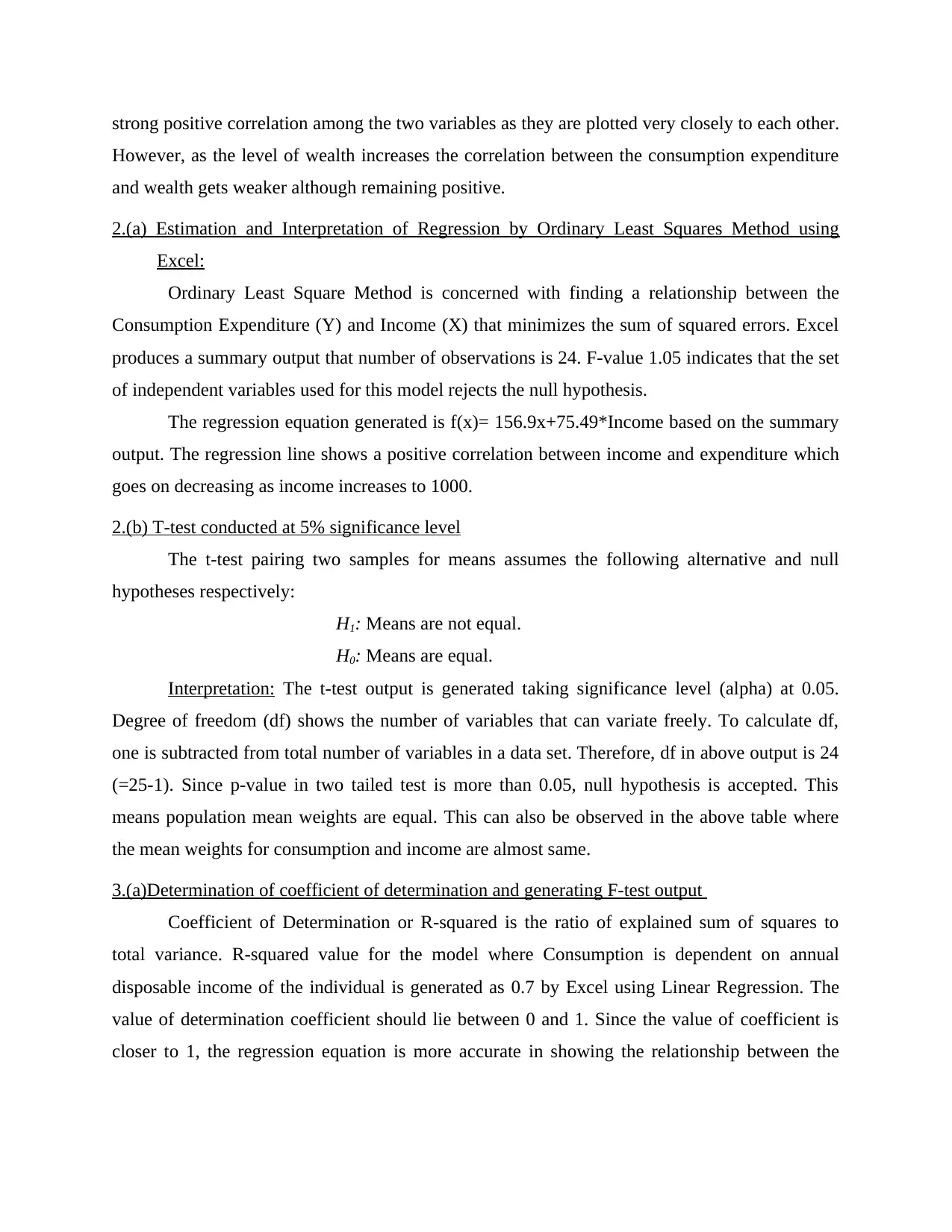
2.(a) Estimation and Interpretation of Regression by Ordinary Least Squares Method using
Excel:
Ordinary Least Square Method is concerned with finding a relationship between the
Consumption Expenditure (Y) and Income (X) that minimizes the sum of squared errors. Excel
produces a summary output that number of observations is 24. F-value 1.05 indicates that the set
of independent variables used for this model rejects the null hypothesis.
The regression equation generated is f(x)= 156.9x+75.49*Income based on the summary
output. The regression line shows a positive correlation between income and expenditure which
goes on decreasing as income increases to 1000.
2.(b) T-test conducted at 5% significance level
The t-test pairing two samples for means assumes the following alternative and null
hypotheses respectively:
H1: Means are not equal.
H0: Means are equal.
Interpretation: The t-test output is generated taking significance level (alpha) at 0.05.
Degree of freedom (df) shows the number of variables that can variate freely. To calculate df,
one is subtracted from total number of variables in a data set. Therefore, df in above output is 24
(=25-1). Since p-value in two tailed test is more than 0.05, null hypothesis is accepted. This
means population mean weights are equal. This can also be observed in the above table where
the mean weights for consumption and income are almost same.
3.(a)Determination of coefficient of determination and generating F-test output
Coefficient of Determination or R-squared is the ratio of explained sum of squares to
total variance. R-squared value for the model where Consumption is dependent on annual
disposable income of the individual is generated as 0.7 by Excel using Linear Regression. The
value of determination coefficient should lie between 0 and 1. Since the value of coefficient is
closer to 1, the regression equation is more accurate in showing the relationship between the
However, as the level of wealth increases the correlation between the consumption expenditure
and wealth gets weaker although remaining positive.
2.(a) Estimation and Interpretation of Regression by Ordinary Least Squares Method using
Excel:
Ordinary Least Square Method is concerned with finding a relationship between the
Consumption Expenditure (Y) and Income (X) that minimizes the sum of squared errors. Excel
produces a summary output that number of observations is 24. F-value 1.05 indicates that the set
of independent variables used for this model rejects the null hypothesis.
The regression equation generated is f(x)= 156.9x+75.49*Income based on the summary
output. The regression line shows a positive correlation between income and expenditure which
goes on decreasing as income increases to 1000.
2.(b) T-test conducted at 5% significance level
The t-test pairing two samples for means assumes the following alternative and null
hypotheses respectively:
H1: Means are not equal.
H0: Means are equal.
Interpretation: The t-test output is generated taking significance level (alpha) at 0.05.
Degree of freedom (df) shows the number of variables that can variate freely. To calculate df,
one is subtracted from total number of variables in a data set. Therefore, df in above output is 24
(=25-1). Since p-value in two tailed test is more than 0.05, null hypothesis is accepted. This
means population mean weights are equal. This can also be observed in the above table where
the mean weights for consumption and income are almost same.
3.(a)Determination of coefficient of determination and generating F-test output
Coefficient of Determination or R-squared is the ratio of explained sum of squares to
total variance. R-squared value for the model where Consumption is dependent on annual
disposable income of the individual is generated as 0.7 by Excel using Linear Regression. The
value of determination coefficient should lie between 0 and 1. Since the value of coefficient is
closer to 1, the regression equation is more accurate in showing the relationship between the
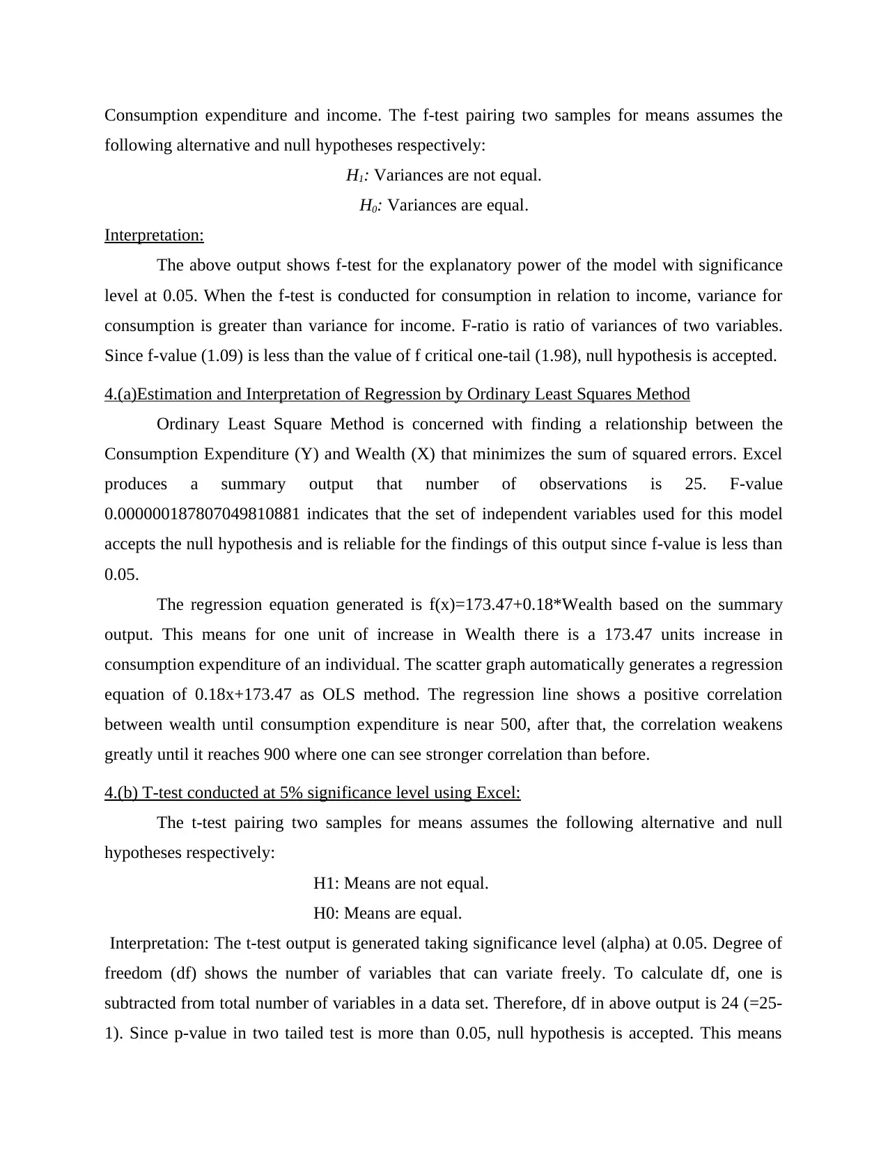
Consumption expenditure and income. The f-test pairing two samples for means assumes the
following alternative and null hypotheses respectively:
H1: Variances are not equal.
H0: Variances are equal.
Interpretation:
The above output shows f-test for the explanatory power of the model with significance
level at 0.05. When the f-test is conducted for consumption in relation to income, variance for
consumption is greater than variance for income. F-ratio is ratio of variances of two variables.
Since f-value (1.09) is less than the value of f critical one-tail (1.98), null hypothesis is accepted.
4.(a)Estimation and Interpretation of Regression by Ordinary Least Squares Method
Ordinary Least Square Method is concerned with finding a relationship between the
Consumption Expenditure (Y) and Wealth (X) that minimizes the sum of squared errors. Excel
produces a summary output that number of observations is 25. F-value
0.000000187807049810881 indicates that the set of independent variables used for this model
accepts the null hypothesis and is reliable for the findings of this output since f-value is less than
0.05.
The regression equation generated is f(x)=173.47+0.18*Wealth based on the summary
output. This means for one unit of increase in Wealth there is a 173.47 units increase in
consumption expenditure of an individual. The scatter graph automatically generates a regression
equation of 0.18x+173.47 as OLS method. The regression line shows a positive correlation
between wealth until consumption expenditure is near 500, after that, the correlation weakens
greatly until it reaches 900 where one can see stronger correlation than before.
4.(b) T-test conducted at 5% significance level using Excel:
The t-test pairing two samples for means assumes the following alternative and null
hypotheses respectively:
H1: Means are not equal.
H0: Means are equal.
Interpretation: The t-test output is generated taking significance level (alpha) at 0.05. Degree of
freedom (df) shows the number of variables that can variate freely. To calculate df, one is
subtracted from total number of variables in a data set. Therefore, df in above output is 24 (=25-
1). Since p-value in two tailed test is more than 0.05, null hypothesis is accepted. This means
⊘ This is a preview!⊘
Do you want full access?
Subscribe today to unlock all pages.
Trusted by 1+ million students worldwide
population mean weights are equal. This can also be observed in the above table where the mean
weights for consumption and income are almost same.
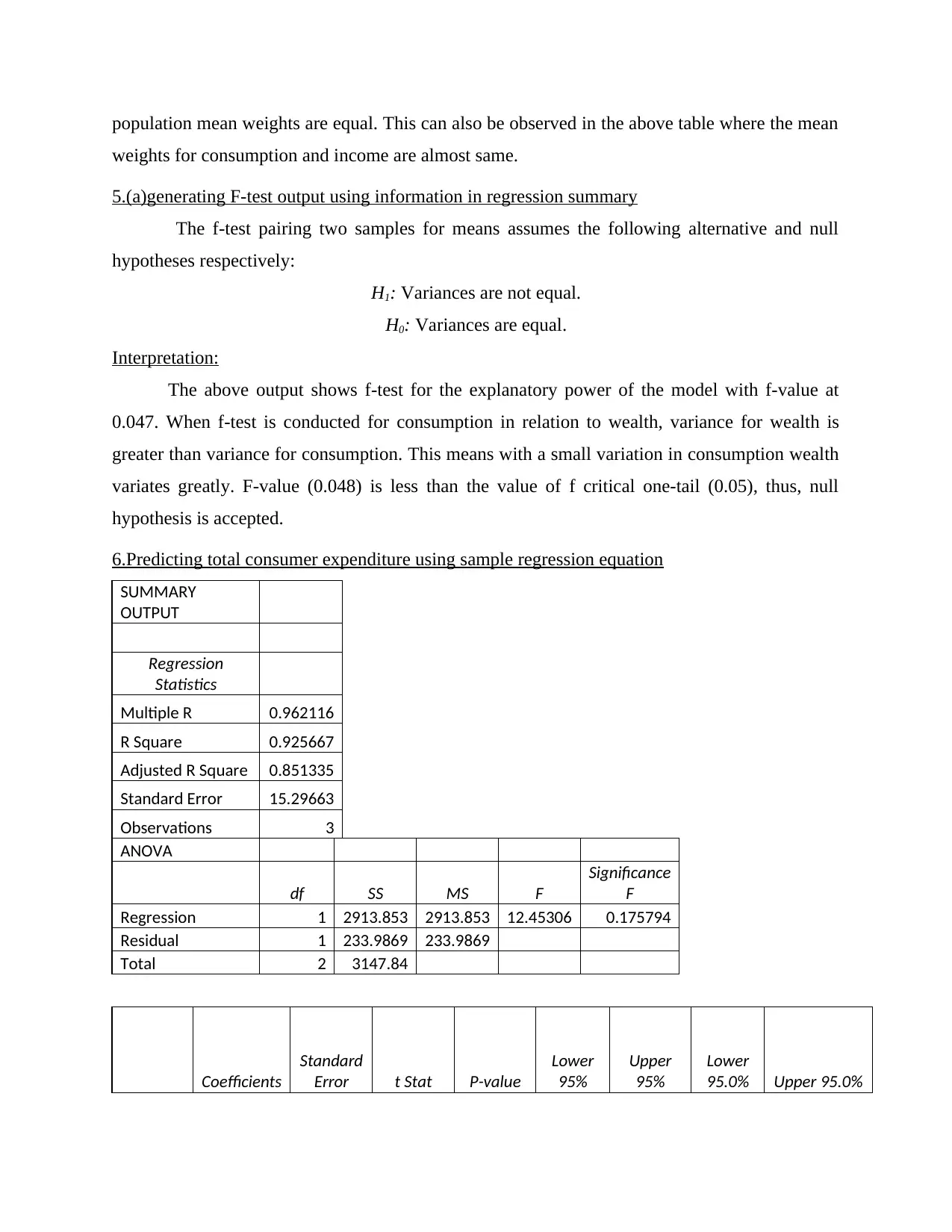
5.(a)generating F-test output using information in regression summary
The f-test pairing two samples for means assumes the following alternative and null
hypotheses respectively:
H1: Variances are not equal.
H0: Variances are equal.
Interpretation:
The above output shows f-test for the explanatory power of the model with f-value at
0.047. When f-test is conducted for consumption in relation to wealth, variance for wealth is
greater than variance for consumption. This means with a small variation in consumption wealth
variates greatly. F-value (0.048) is less than the value of f critical one-tail (0.05), thus, null
hypothesis is accepted.
6.Predicting total consumer expenditure using sample regression equation
SUMMARY
OUTPUT
Regression
Statistics
Multiple R 0.962116
R Square 0.925667
Adjusted R Square 0.851335
Standard Error 15.29663
Observations 3
ANOVA
df SS MS F
Significance
F
Regression 1 2913.853 2913.853 12.45306 0.175794
Residual 1 233.9869 233.9869
Total 2 3147.84
Coefficients
Standard
Error t Stat P-value
Lower
95%
Upper
95%
Lower
95.0% Upper 95.0%
weights for consumption and income are almost same.
5.(a)generating F-test output using information in regression summary
The f-test pairing two samples for means assumes the following alternative and null
hypotheses respectively:
H1: Variances are not equal.
H0: Variances are equal.
Interpretation:
The above output shows f-test for the explanatory power of the model with f-value at
0.047. When f-test is conducted for consumption in relation to wealth, variance for wealth is
greater than variance for consumption. This means with a small variation in consumption wealth
variates greatly. F-value (0.048) is less than the value of f critical one-tail (0.05), thus, null
hypothesis is accepted.
6.Predicting total consumer expenditure using sample regression equation
SUMMARY
OUTPUT
Regression
Statistics
Multiple R 0.962116
R Square 0.925667
Adjusted R Square 0.851335
Standard Error 15.29663
Observations 3
ANOVA
df SS MS F
Significance
F
Regression 1 2913.853 2913.853 12.45306 0.175794
Residual 1 233.9869 233.9869
Total 2 3147.84
Coefficients
Standard
Error t Stat P-value
Lower
95%
Upper
95%
Lower
95.0% Upper 95.0%
Paraphrase This Document
Need a fresh take? Get an instant paraphrase of this document with our AI Paraphraser
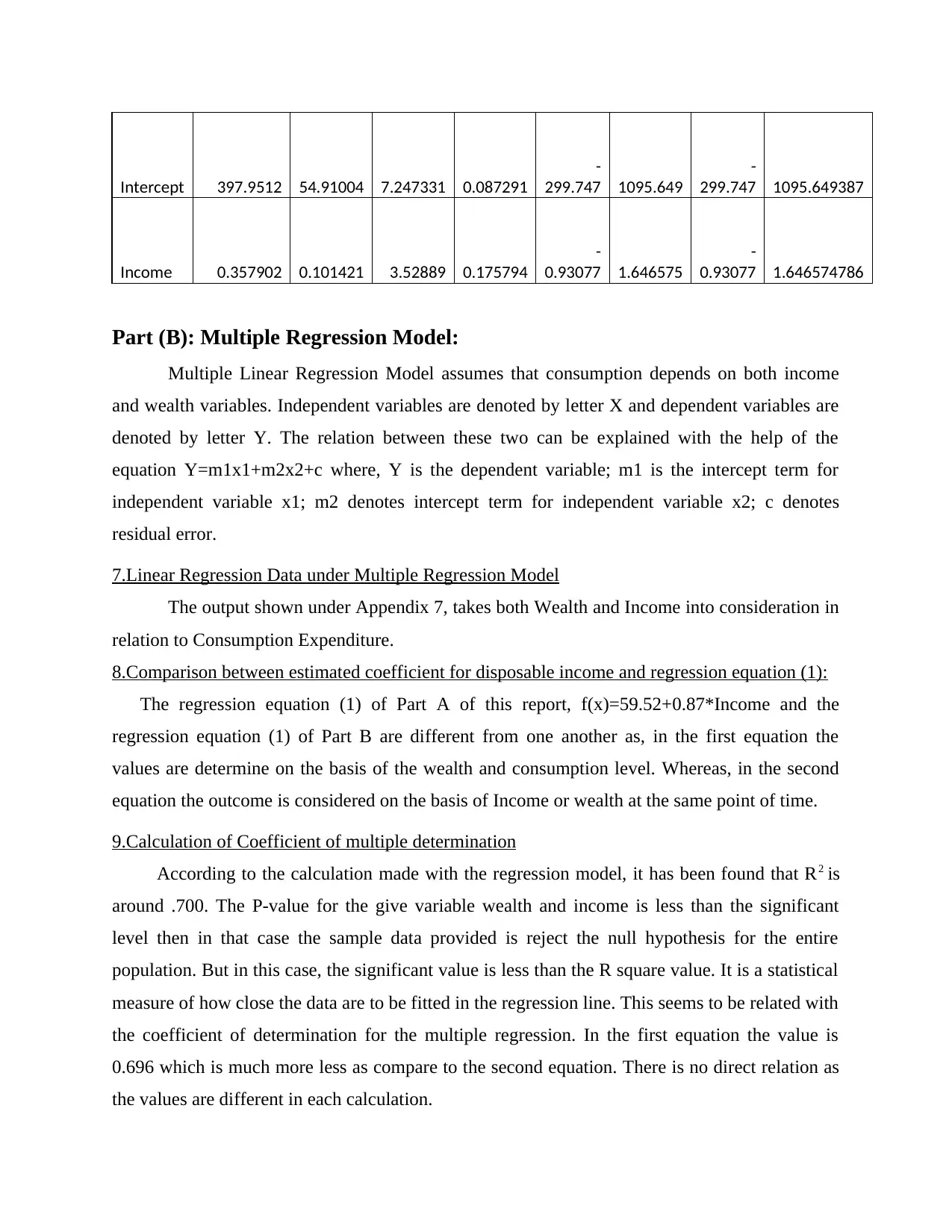
Intercept 397.9512 54.91004 7.247331 0.087291
-
299.747 1095.649
-
299.747 1095.649387
Income 0.357902 0.101421 3.52889 0.175794
-
0.93077 1.646575
-
0.93077 1.646574786
Part (B): Multiple Regression Model:
Multiple Linear Regression Model assumes that consumption depends on both income
and wealth variables. Independent variables are denoted by letter X and dependent variables are
denoted by letter Y. The relation between these two can be explained with the help of the
equation Y=m1x1+m2x2+c where, Y is the dependent variable; m1 is the intercept term for
independent variable x1; m2 denotes intercept term for independent variable x2; c denotes
residual error.
7.Linear Regression Data under Multiple Regression Model
The output shown under Appendix 7, takes both Wealth and Income into consideration in
relation to Consumption Expenditure.
8.Comparison between estimated coefficient for disposable income and regression equation (1):
The regression equation (1) of Part A of this report, f(x)=59.52+0.87*Income and the
regression equation (1) of Part B are different from one another as, in the first equation the
values are determine on the basis of the wealth and consumption level. Whereas, in the second
equation the outcome is considered on the basis of Income or wealth at the same point of time.
9.Calculation of Coefficient of multiple determination
According to the calculation made with the regression model, it has been found that R2 is
around .700. The P-value for the give variable wealth and income is less than the significant
level then in that case the sample data provided is reject the null hypothesis for the entire
population. But in this case, the significant value is less than the R square value. It is a statistical
measure of how close the data are to be fitted in the regression line. This seems to be related with
the coefficient of determination for the multiple regression. In the first equation the value is
0.696 which is much more less as compare to the second equation. There is no direct relation as
the values are different in each calculation.
-
299.747 1095.649
-
299.747 1095.649387
Income 0.357902 0.101421 3.52889 0.175794
-
0.93077 1.646575
-
0.93077 1.646574786
Part (B): Multiple Regression Model:
Multiple Linear Regression Model assumes that consumption depends on both income
and wealth variables. Independent variables are denoted by letter X and dependent variables are
denoted by letter Y. The relation between these two can be explained with the help of the
equation Y=m1x1+m2x2+c where, Y is the dependent variable; m1 is the intercept term for
independent variable x1; m2 denotes intercept term for independent variable x2; c denotes
residual error.
7.Linear Regression Data under Multiple Regression Model
The output shown under Appendix 7, takes both Wealth and Income into consideration in
relation to Consumption Expenditure.
8.Comparison between estimated coefficient for disposable income and regression equation (1):
The regression equation (1) of Part A of this report, f(x)=59.52+0.87*Income and the
regression equation (1) of Part B are different from one another as, in the first equation the
values are determine on the basis of the wealth and consumption level. Whereas, in the second
equation the outcome is considered on the basis of Income or wealth at the same point of time.
9.Calculation of Coefficient of multiple determination
According to the calculation made with the regression model, it has been found that R2 is
around .700. The P-value for the give variable wealth and income is less than the significant
level then in that case the sample data provided is reject the null hypothesis for the entire
population. But in this case, the significant value is less than the R square value. It is a statistical
measure of how close the data are to be fitted in the regression line. This seems to be related with
the coefficient of determination for the multiple regression. In the first equation the value is
0.696 which is much more less as compare to the second equation. There is no direct relation as
the values are different in each calculation.
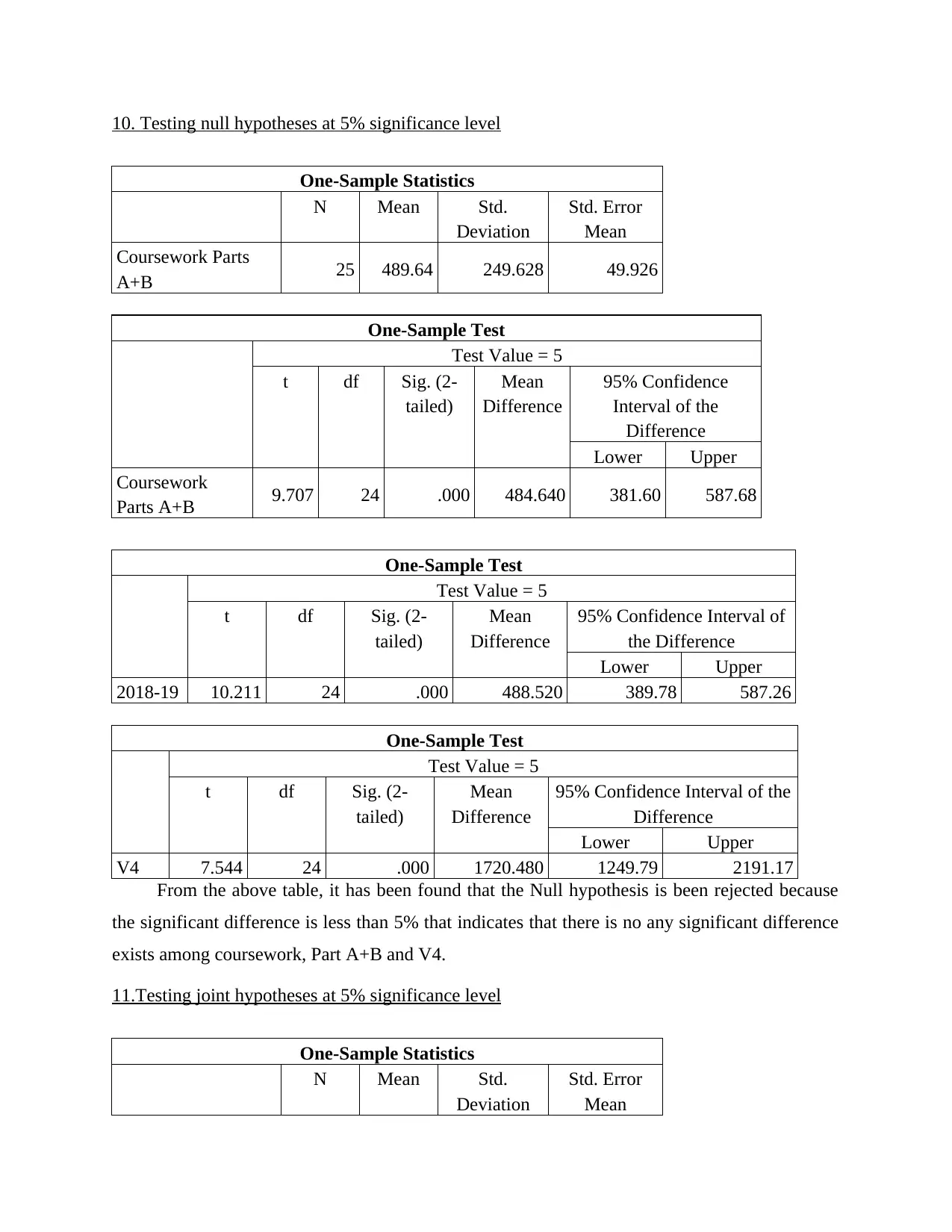
10. Testing null hypotheses at 5% significance level
One-Sample Statistics
N Mean Std.
Deviation
Std. Error
Mean
Coursework Parts
A+B 25 489.64 249.628 49.926
One-Sample Test
Test Value = 5
t df Sig. (2-
tailed)
Mean
Difference
95% Confidence
Interval of the
Difference
Lower Upper
Coursework
Parts A+B 9.707 24 .000 484.640 381.60 587.68
One-Sample Test
Test Value = 5
t df Sig. (2-
tailed)
Mean
Difference
95% Confidence Interval of
the Difference
Lower Upper
2018-19 10.211 24 .000 488.520 389.78 587.26
One-Sample Test
Test Value = 5
t df Sig. (2-
tailed)
Mean
Difference
95% Confidence Interval of the
Difference
Lower Upper
V4 7.544 24 .000 1720.480 1249.79 2191.17
From the above table, it has been found that the Null hypothesis is been rejected because
the significant difference is less than 5% that indicates that there is no any significant difference
exists among coursework, Part A+B and V4.
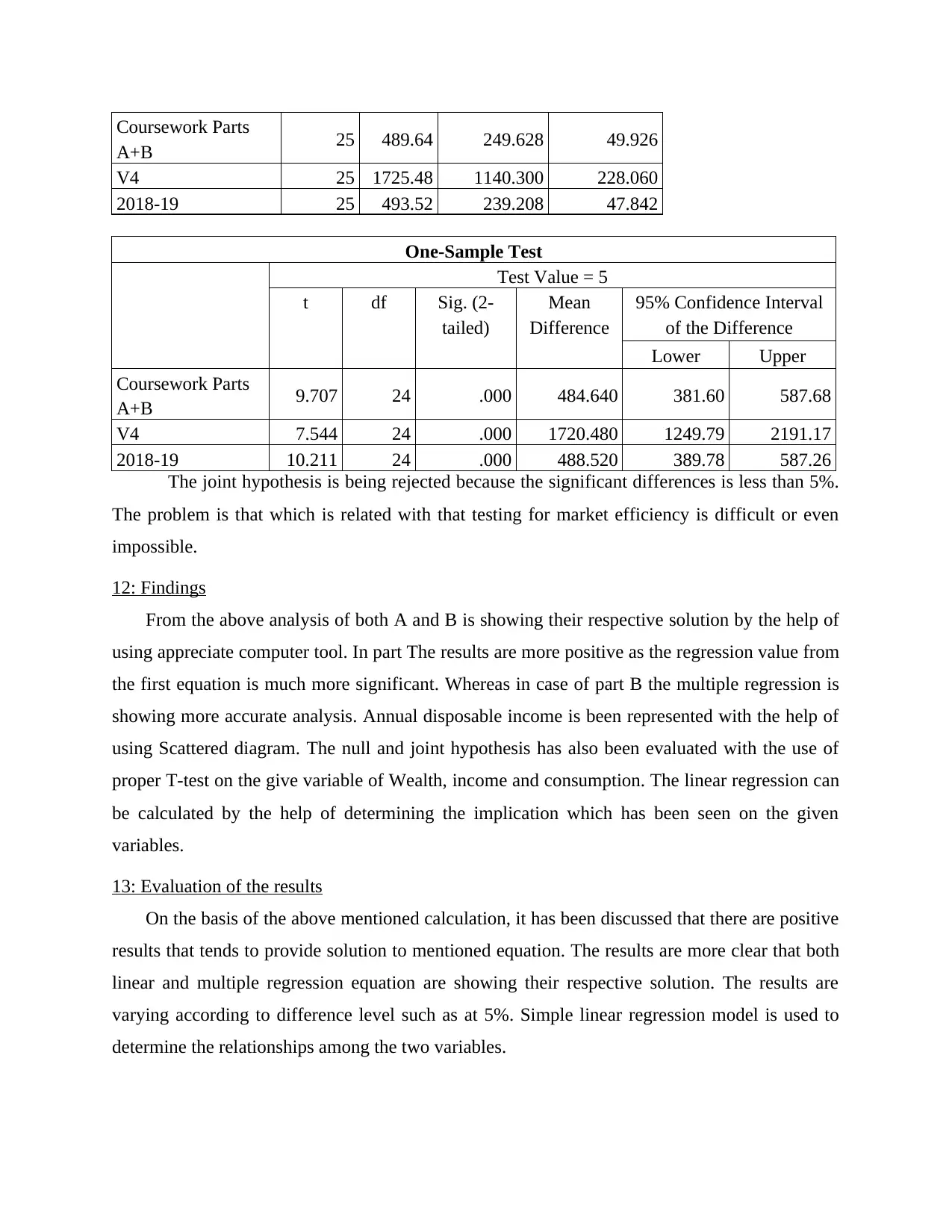
11.Testing joint hypotheses at 5% significance level
One-Sample Statistics
N Mean Std.
Deviation
Std. Error
Mean
One-Sample Statistics
N Mean Std.
Deviation
Std. Error
Mean
Coursework Parts
A+B 25 489.64 249.628 49.926
One-Sample Test
Test Value = 5
t df Sig. (2-
tailed)
Mean
Difference
95% Confidence
Interval of the
Difference
Lower Upper
Coursework
Parts A+B 9.707 24 .000 484.640 381.60 587.68
One-Sample Test
Test Value = 5
t df Sig. (2-
tailed)
Mean
Difference
95% Confidence Interval of
the Difference
Lower Upper
2018-19 10.211 24 .000 488.520 389.78 587.26
One-Sample Test
Test Value = 5
t df Sig. (2-
tailed)
Mean
Difference
95% Confidence Interval of the
Difference
Lower Upper
V4 7.544 24 .000 1720.480 1249.79 2191.17
From the above table, it has been found that the Null hypothesis is been rejected because
the significant difference is less than 5% that indicates that there is no any significant difference
exists among coursework, Part A+B and V4.
11.Testing joint hypotheses at 5% significance level
One-Sample Statistics
N Mean Std.
Deviation
Std. Error
Mean
⊘ This is a preview!⊘
Do you want full access?
Subscribe today to unlock all pages.
Trusted by 1+ million students worldwide
Coursework Parts
A+B 25 489.64 249.628 49.926
V4 25 1725.48 1140.300 228.060
2018-19 25 493.52 239.208 47.842
One-Sample Test
Test Value = 5
t df Sig. (2-
tailed)
Mean
Difference
95% Confidence Interval
of the Difference
Lower Upper
Coursework Parts
A+B 9.707 24 .000 484.640 381.60 587.68
V4 7.544 24 .000 1720.480 1249.79 2191.17
2018-19 10.211 24 .000 488.520 389.78 587.26
The joint hypothesis is being rejected because the significant differences is less than 5%.
The problem is that which is related with that testing for market efficiency is difficult or even
impossible.
12: Findings
From the above analysis of both A and B is showing their respective solution by the help of
using appreciate computer tool. In part The results are more positive as the regression value from
the first equation is much more significant. Whereas in case of part B the multiple regression is
showing more accurate analysis. Annual disposable income is been represented with the help of
using Scattered diagram. The null and joint hypothesis has also been evaluated with the use of
proper T-test on the give variable of Wealth, income and consumption. The linear regression can
be calculated by the help of determining the implication which has been seen on the given
variables.
13: Evaluation of the results
On the basis of the above mentioned calculation, it has been discussed that there are positive
results that tends to provide solution to mentioned equation. The results are more clear that both
linear and multiple regression equation are showing their respective solution. The results are
varying according to difference level such as at 5%. Simple linear regression model is used to
determine the relationships among the two variables.
Paraphrase This Document
Need a fresh take? Get an instant paraphrase of this document with our AI Paraphraser
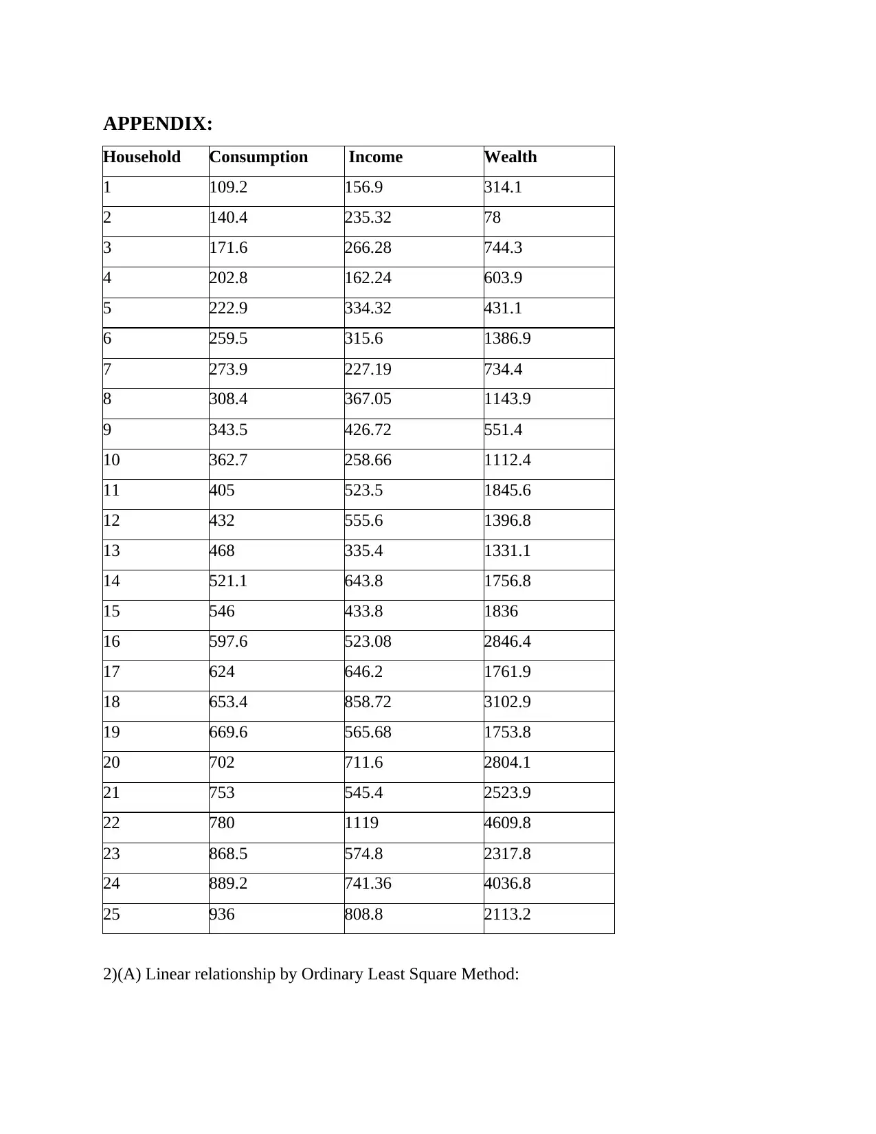
APPENDIX:
Household Consumption Income Wealth
1 109.2 156.9 314.1
2 140.4 235.32 78
3 171.6 266.28 744.3
4 202.8 162.24 603.9
5 222.9 334.32 431.1
6 259.5 315.6 1386.9
7 273.9 227.19 734.4
8 308.4 367.05 1143.9
9 343.5 426.72 551.4
10 362.7 258.66 1112.4
11 405 523.5 1845.6
12 432 555.6 1396.8
13 468 335.4 1331.1
14 521.1 643.8 1756.8
15 546 433.8 1836
16 597.6 523.08 2846.4
17 624 646.2 1761.9
18 653.4 858.72 3102.9
19 669.6 565.68 1753.8
20 702 711.6 2804.1
21 753 545.4 2523.9
22 780 1119 4609.8
23 868.5 574.8 2317.8
24 889.2 741.36 4036.8
25 936 808.8 2113.2
2)(A) Linear relationship by Ordinary Least Square Method:
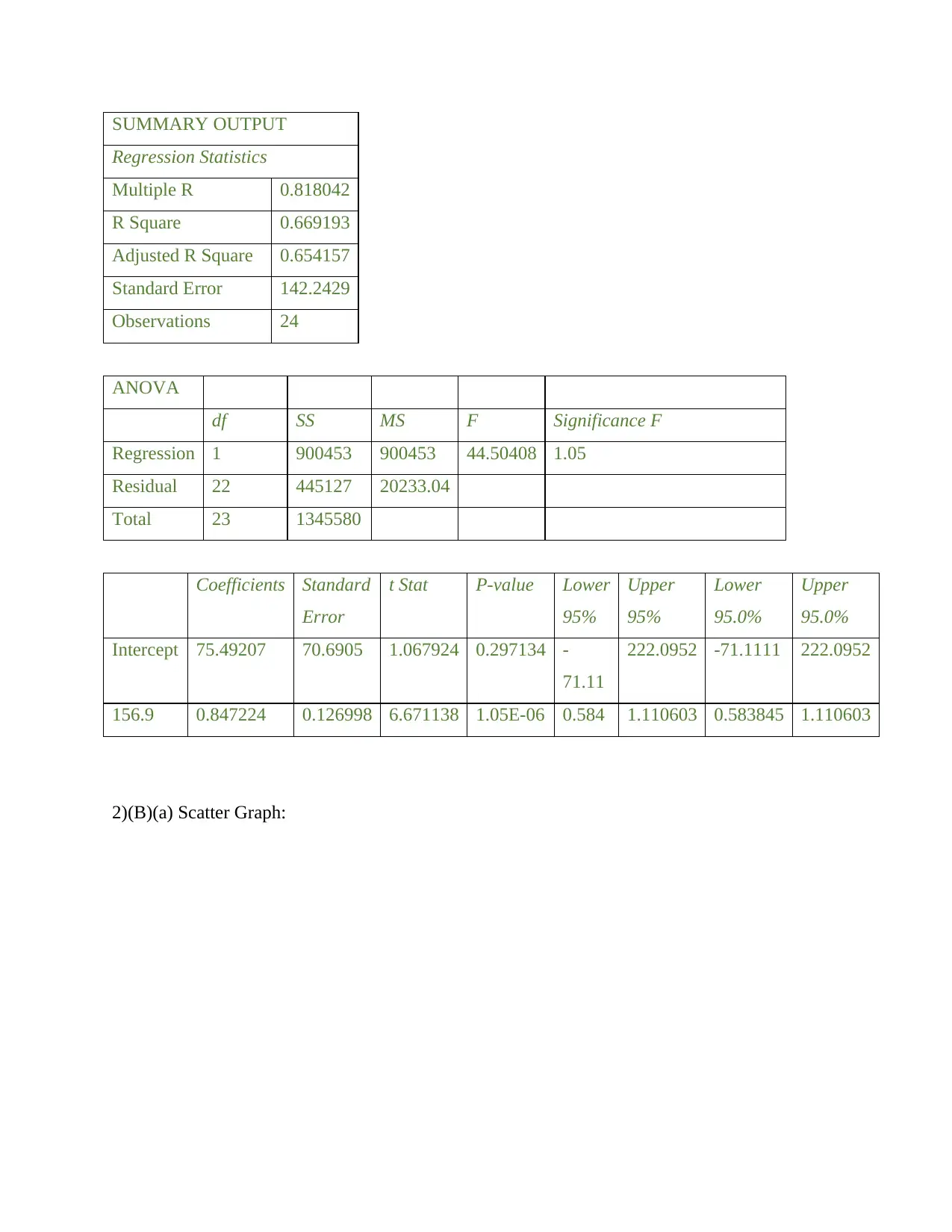
SUMMARY OUTPUT
Regression Statistics
Multiple R 0.818042
R Square 0.669193
Adjusted R Square 0.654157
Standard Error 142.2429
Observations 24
ANOVA
df SS MS F Significance F
Regression 1 900453 900453 44.50408 1.05
Residual 22 445127 20233.04
Total 23 1345580
Coefficients Standard
Error
t Stat P-value Lower
95%
Upper
95%
Lower
95.0%
Upper
95.0%
Intercept 75.49207 70.6905 1.067924 0.297134 -
71.11
222.0952 -71.1111 222.0952
156.9 0.847224 0.126998 6.671138 1.05E-06 0.584 1.110603 0.583845 1.110603
2)(B)(a) Scatter Graph:
⊘ This is a preview!⊘
Do you want full access?
Subscribe today to unlock all pages.
Trusted by 1+ million students worldwide
1 out of 16
Related Documents


Your All-in-One AI-Powered Toolkit for Academic Success.
+13062052269
info@desklib.com
Available 24*7 on WhatsApp / Email
![[object Object]](/_next/static/media/star-bottom.7253800d.svg)
Unlock your academic potential
Copyright © 2020–2026 A2Z Services. All Rights Reserved. Developed and managed by ZUCOL.