Econometrics: Demand, Supply, Probit, and Logit Models Analysis

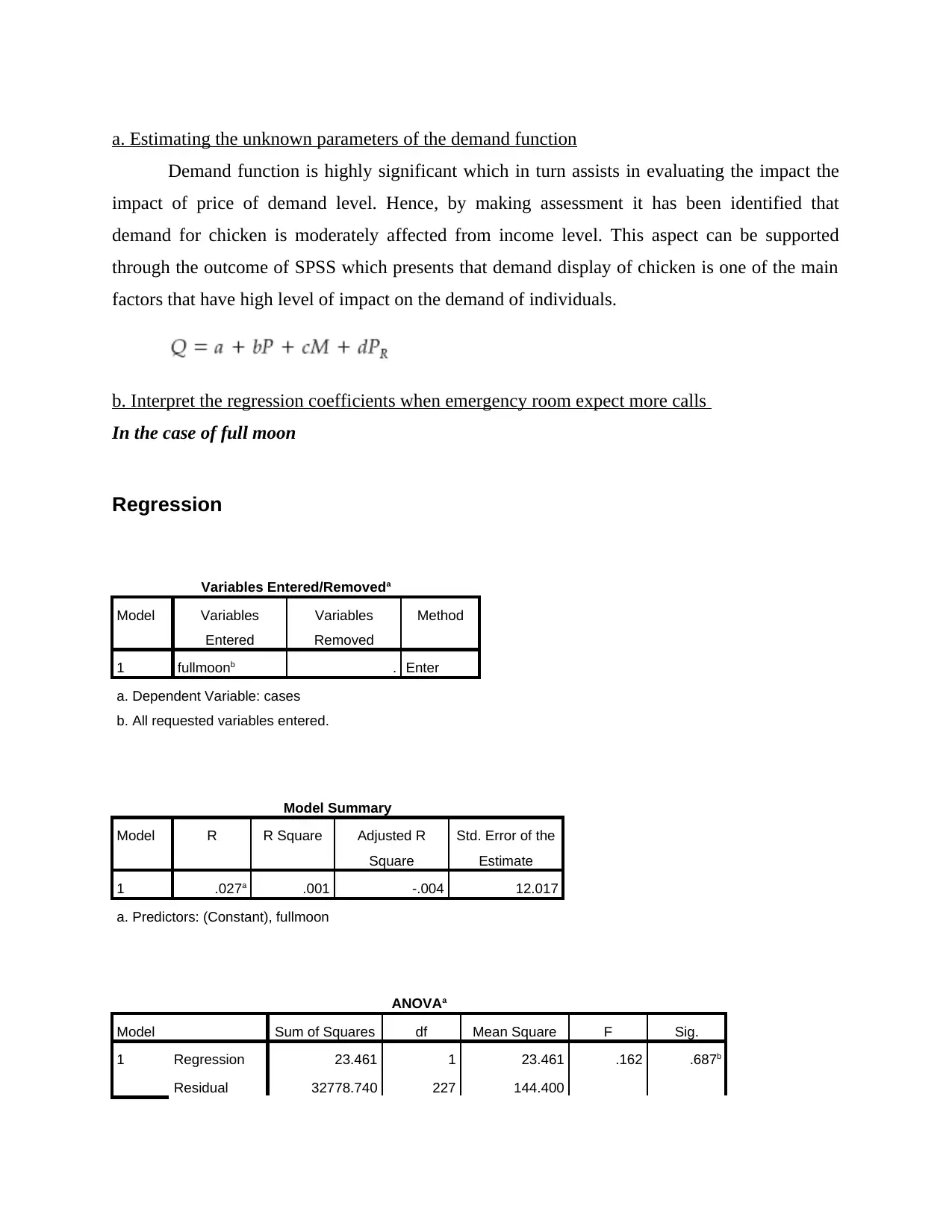
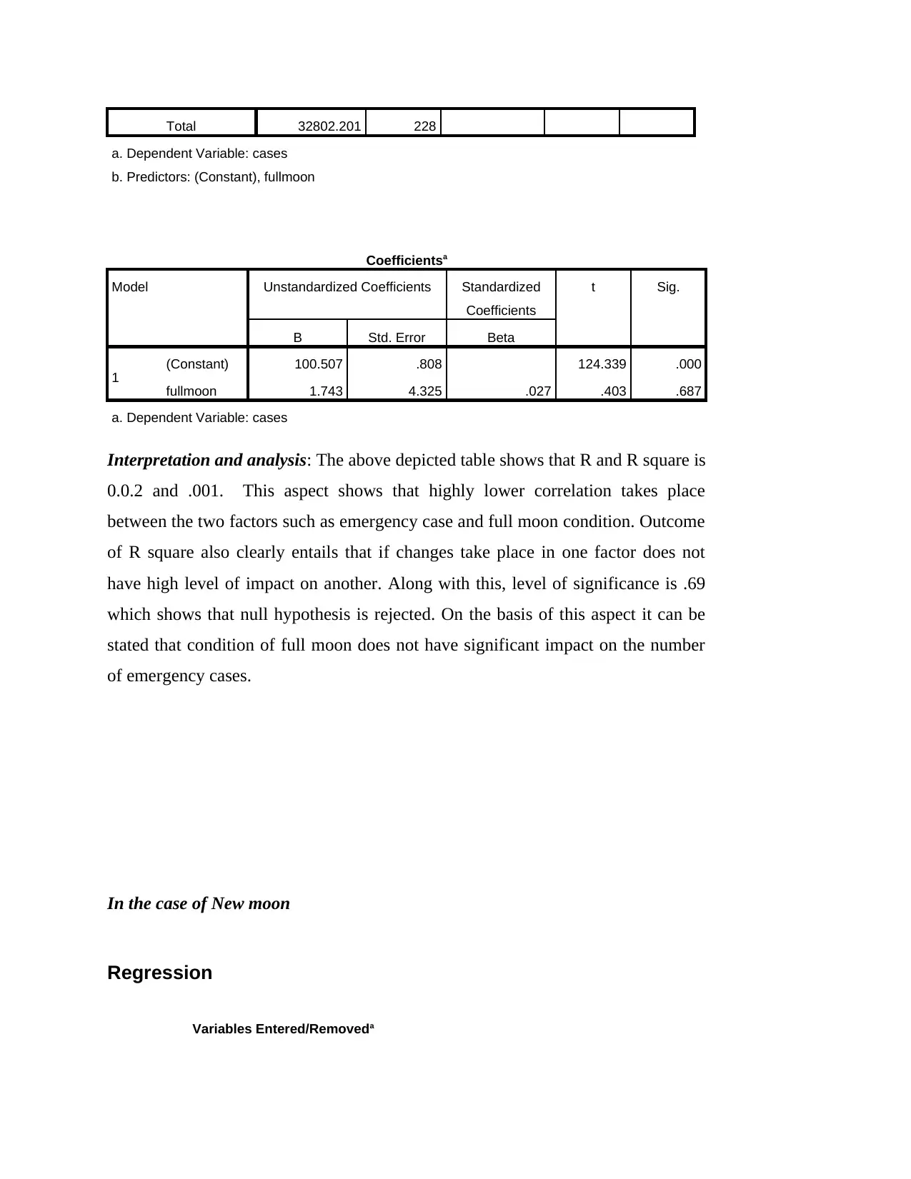
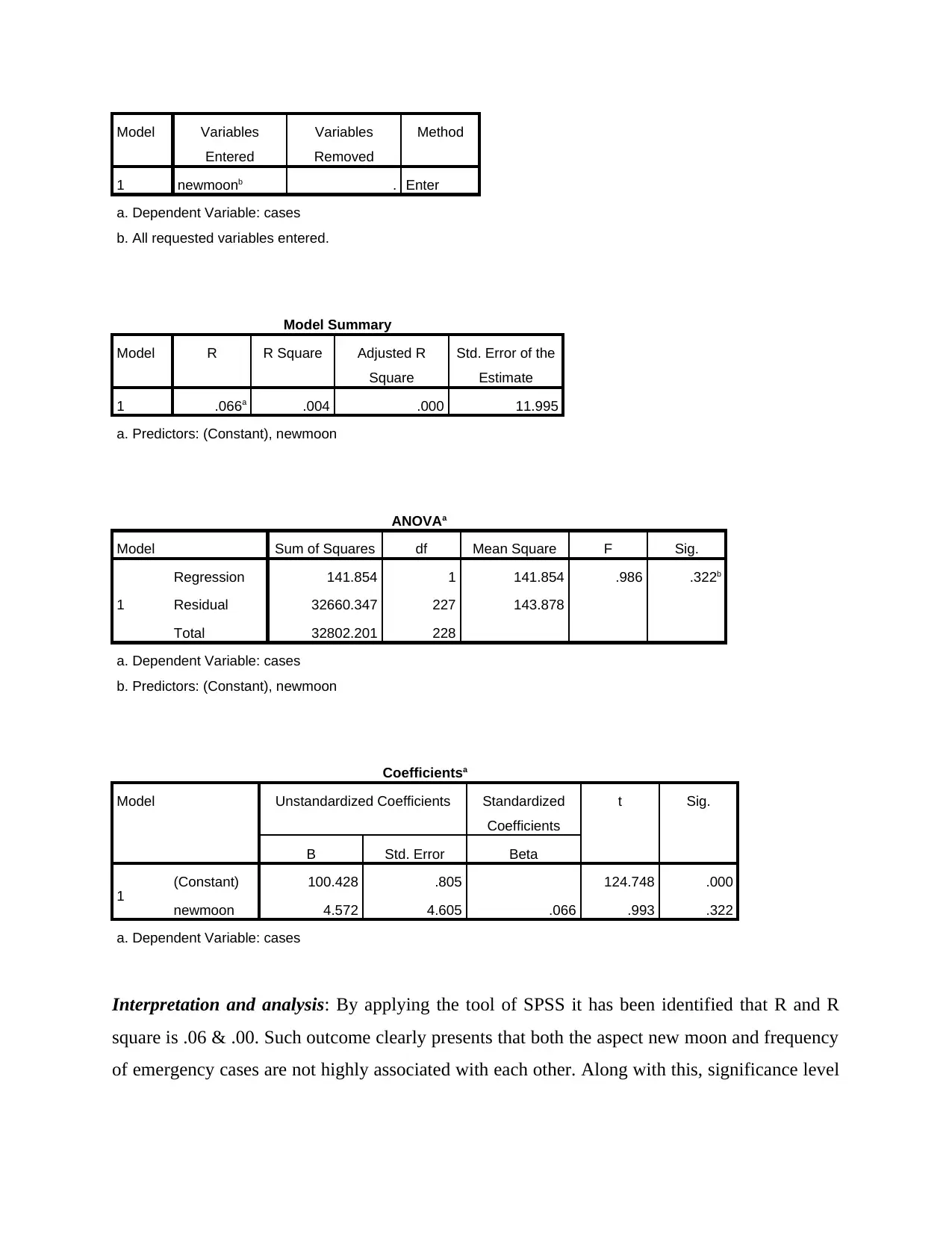
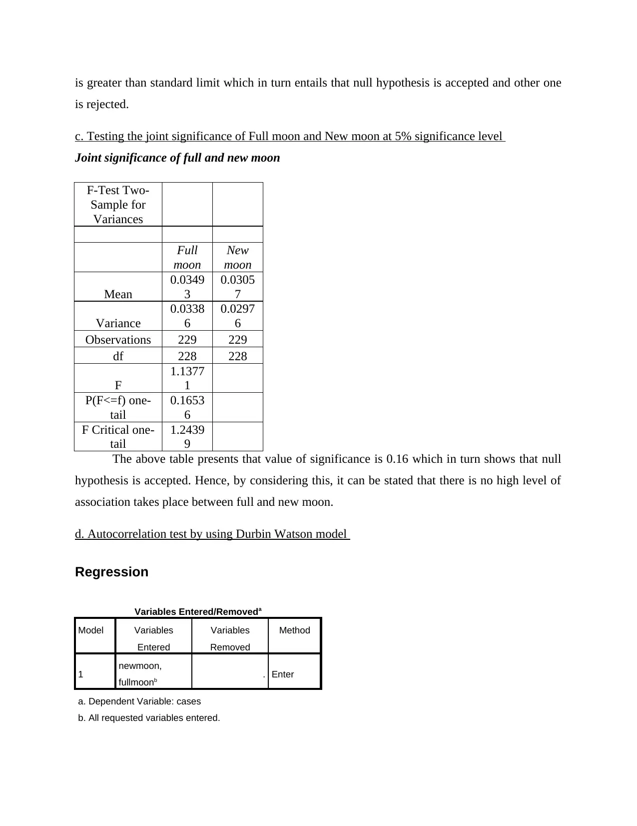
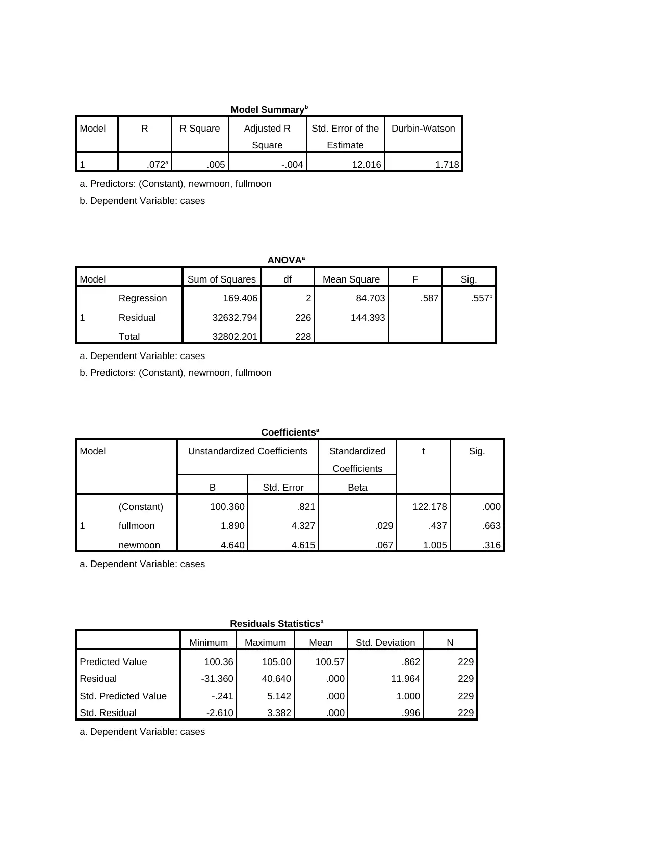
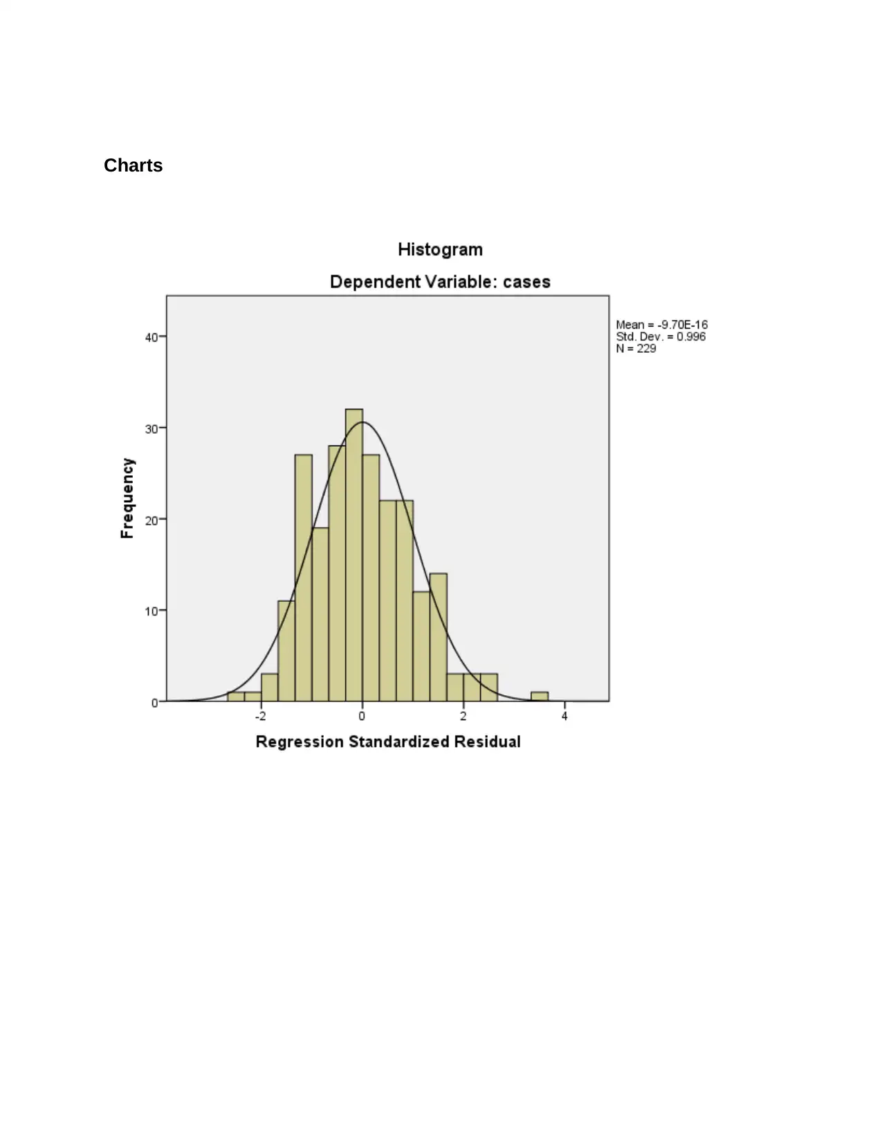
This econometrics assignment delves into various economic models and statistical techniques. It begins by estimating demand functions and interpreting regression coefficients in the context of emergency room calls and moon phases. It then tests for joint significance and autocorrelation using the Durbin-Watson model, followed by re-estimation after correcting for autocorrelation. The assignment continues with estimating a supply equation using the least squares method and testing beliefs with the Hausman test, before using an instrumental variables estimator. Finally, it explores probit and logit models with outcome variables, including descriptive statistics, frequency tables, and parameter estimates, all analyzed using SPSS. The assignment provides detailed interpretations of the results and statistical outputs, offering a comprehensive understanding of econometric methods.

Econometric

Table of Contents
a. Estimating the unknown parameters of the demand function..................................................3
b. Interpret the regression coefficients when emergency room expect more calls......................3
c. Testing the joint significance of Full moon and New moon at 5% significance level............6
d. Autocorrelation test by using Durbin Watson model..............................................................6
e. Re-estimating the model after correcting for autocorrelation................................................10
QUESTION 2................................................................................................................................10
a. Estimating supply equation by least square method..............................................................10
b. Using Hausman to test to examine this belief at 5% level of significance............................12
c. Estimating supply equation using an instrumental variables estimator with all available
instruments.................................................................................................................................12
QUESTION 3................................................................................................................................12
a. Estimating a probit model with outcome...............................................................................12
b. Using logit model with outcome variable..............................................................................17

a. Estimating the unknown parameters of the demand function
Demand function is highly significant which in turn assists in evaluating the impact the
impact of price of demand level. Hence, by making assessment it has been identified that
demand for chicken is moderately affected from income level. This aspect can be supported
through the outcome of SPSS which presents that demand display of chicken is one of the main
factors that have high level of impact on the demand of individuals.
b. Interpret the regression coefficients when emergency room expect more calls
In the case of full moon
Regression
Variables Entered/Removeda
Model Variables
Entered
Variables
Removed
Method
1 fullmoonb . Enter
a. Dependent Variable: cases
b. All requested variables entered.
Model Summary
Model R R Square Adjusted R
Square
Std. Error of the
Estimate
1 .027a .001 -.004 12.017
a. Predictors: (Constant), fullmoon
ANOVAa
Model Sum of Squares df Mean Square F Sig.
1 Regression 23.461 1 23.461 .162 .687b
Residual 32778.740 227 144.400

Total 32802.201 228
a. Dependent Variable: cases
b. Predictors: (Constant), fullmoon
Coefficientsa
Model Unstandardized Coefficients Standardized
Coefficients
t Sig.
B Std. Error Beta
1 (Constant) 100.507 .808 124.339 .000
fullmoon 1.743 4.325 .027 .403 .687
a. Dependent Variable: cases
Interpretation and analysis: The above depicted table shows that R and R square is
0.0.2 and .001. This aspect shows that highly lower correlation takes place
between the two factors such as emergency case and full moon condition. Outcome
of R square also clearly entails that if changes take place in one factor does not
have high level of impact on another. Along with this, level of significance is .69
which shows that null hypothesis is rejected. On the basis of this aspect it can be
stated that condition of full moon does not have significant impact on the number
of emergency cases.
In the case of New moon
Regression
Variables Entered/Removeda

Model Variables
Entered
Variables
Removed
Method
1 newmoonb . Enter
a. Dependent Variable: cases
b. All requested variables entered.
Model Summary
Model R R Square Adjusted R
Square
Std. Error of the
Estimate
1 .066a .004 .000 11.995
a. Predictors: (Constant), newmoon
ANOVAa
Model Sum of Squares df Mean Square F Sig.
1
Regression 141.854 1 141.854 .986 .322b
Residual 32660.347 227 143.878
Total 32802.201 228
a. Dependent Variable: cases
b. Predictors: (Constant), newmoon
Coefficientsa
Model Unstandardized Coefficients Standardized
Coefficients
t Sig.
B Std. Error Beta
1 (Constant) 100.428 .805 124.748 .000
newmoon 4.572 4.605 .066 .993 .322
a. Dependent Variable: cases
Interpretation and analysis: By applying the tool of SPSS it has been identified that R and R
square is .06 & .00. Such outcome clearly presents that both the aspect new moon and frequency
of emergency cases are not highly associated with each other. Along with this, significance level

is greater than standard limit which in turn entails that null hypothesis is accepted and other one
is rejected.
c. Testing the joint significance of Full moon and New moon at 5% significance level
Joint significance of full and new moon
F-Test Two-
Sample for
Variances
Full
moon
New
moon
Mean
0.0349
3
0.0305
7
Variance
0.0338
6
0.0297
6
Observations 229 229
df 228 228
F
1.1377
1
P(F<=f) one-
tail
0.1653
6
F Critical one-
tail
1.2439
9
The above table presents that value of significance is 0.16 which in turn shows that null
hypothesis is accepted. Hence, by considering this, it can be stated that there is no high level of
association takes place between full and new moon.
d. Autocorrelation test by using Durbin Watson model
Regression
Variables Entered/Removeda
Model Variables
Entered
Variables
Removed
Method
1 newmoon,
fullmoonb . Enter
a. Dependent Variable: cases
b. All requested variables entered.

Model Summaryb
Model R R Square Adjusted R
Square
Std. Error of the
Estimate
Durbin-Watson
1 .072a .005 -.004 12.016 1.718
a. Predictors: (Constant), newmoon, fullmoon
b. Dependent Variable: cases
ANOVAa
Model Sum of Squares df Mean Square F Sig.
1
Regression 169.406 2 84.703 .587 .557b
Residual 32632.794 226 144.393
Total 32802.201 228
a. Dependent Variable: cases
b. Predictors: (Constant), newmoon, fullmoon
Coefficientsa
Model Unstandardized Coefficients Standardized
Coefficients
t Sig.
B Std. Error Beta
1
(Constant) 100.360 .821 122.178 .000
fullmoon 1.890 4.327 .029 .437 .663
newmoon 4.640 4.615 .067 1.005 .316
a. Dependent Variable: cases
Residuals Statisticsa
Minimum Maximum Mean Std. Deviation N
Predicted Value 100.36 105.00 100.57 .862 229
Residual -31.360 40.640 .000 11.964 229
Std. Predicted Value -.241 5.142 .000 1.000 229
Std. Residual -2.610 3.382 .000 .996 229
a. Dependent Variable: cases

Charts

e. Re-estimating the model after correcting for autocorrelation
Interpretation of Durbin Watson test: Tabular presentation shows that value of D is 1.72
respectively. In accordance with the rules and regulations autocorrelation can said to be positive
when it lies between 0 to 4 and vice versa. Hence, autocorrelation between full and new moon is
positive to the significant level.
QUESTION 2
a. Estimating supply equation by least square method
QPRD = β1 + β2 In(Pt) + β3 In (PFt) + β4 Time t + Et

Variables Entered/Removeda
Model Variables
Entered
Variables
Removed
Method
1 qb . Enter
a. Dependent Variable: qprod
b. All requested variables entered.
Model Summary
Model R R Square Adjusted R
Square
Std. Error of the
Estimate
1 .979a .959 .958 1146.173
a. Predictors: (Constant), q
ANOVAa
Model Sum of Squares df Mean Square F Sig.
1
Regression 1496691712.44
1 1 1496691712.44
1 1139.284 .000b
Residual 64371929.994 49 1313712.857
Total 1561063642.43
5 50
a. Dependent Variable: qprod
b. Predictors: (Constant), q

Coefficientsa
Model Unstandardized Coefficients Standardized
Coefficients
t Sig.
B Std. Error Beta
1 (Constant) -6479.862 457.034 -14.178 .000
q 469.048 13.896 .979 33.753 .000
a. Dependent Variable: qprod
The above mentioned table shows that level of significance is 0.00. Hence, it can be
stated that consumption of chicken is highly affected from the production level.
b. Using Hausman to test to examine this belief at 5% level of significance
Analysts can check consistency level by making use of Hauman test. Such model
differentiates fixed and random variable in panel data. Hence, in the case of B1 (RE estimator)
null hypothesis is true and vice versa.
H = (B1-B0) [ Var (bo – Var (b1)t] (b1- b0)
c. Estimating supply equation using an instrumental variables estimator with all available
instruments
By using instrumental variables analysts can estimate or determine causal relationship
when controlled experiments are not feasible. Through the means of instrumental variable
estimator correlation between explanatory and dependent variable can easily be assessed. Hence,
by using such technique US department of agriculture can draw suitable equation in the
following manner:
Y = Xβ +U
QUESTION 3
a. Estimating a probit model with outcome
Probit model