Econometrics Assignment: Regression Models and Hypothesis Testing
VerifiedAdded on 2020/04/07
|11
|705
|106
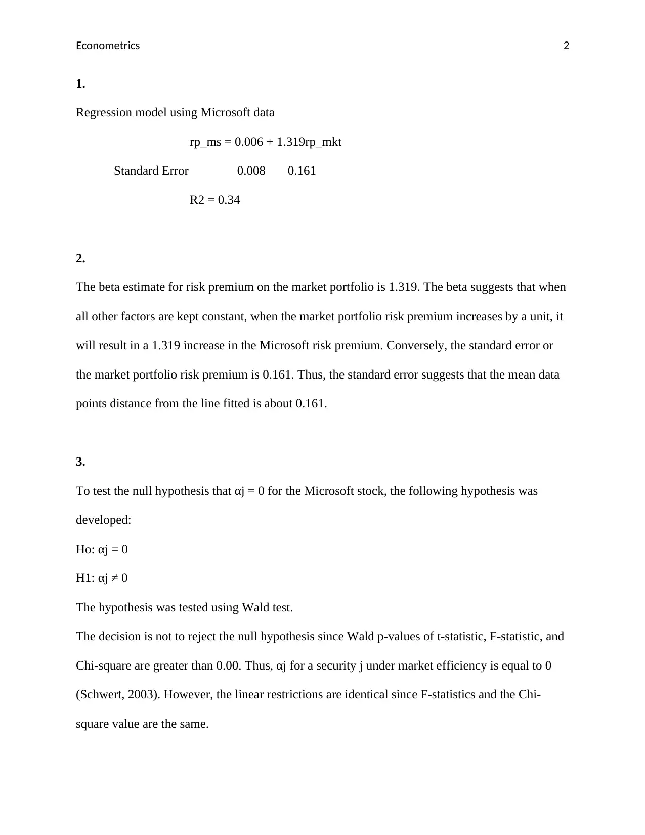
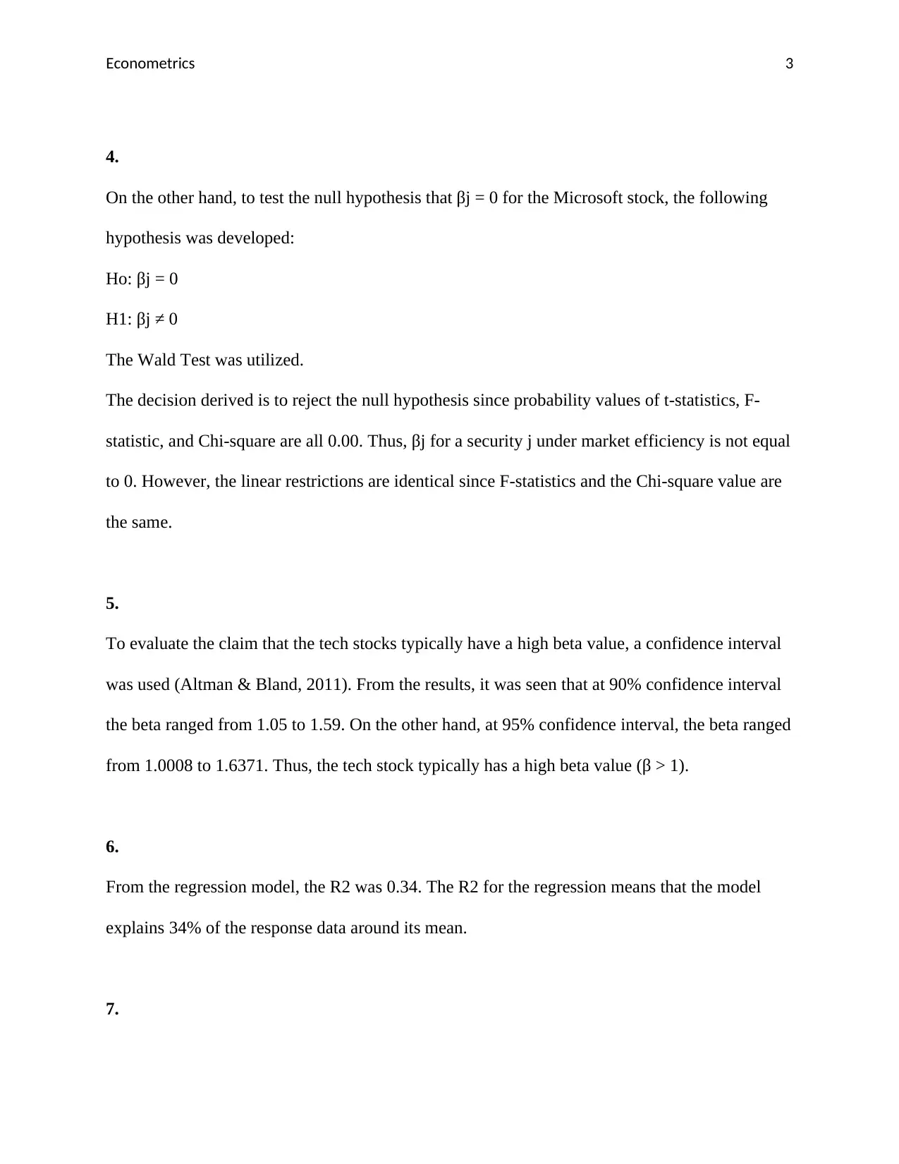
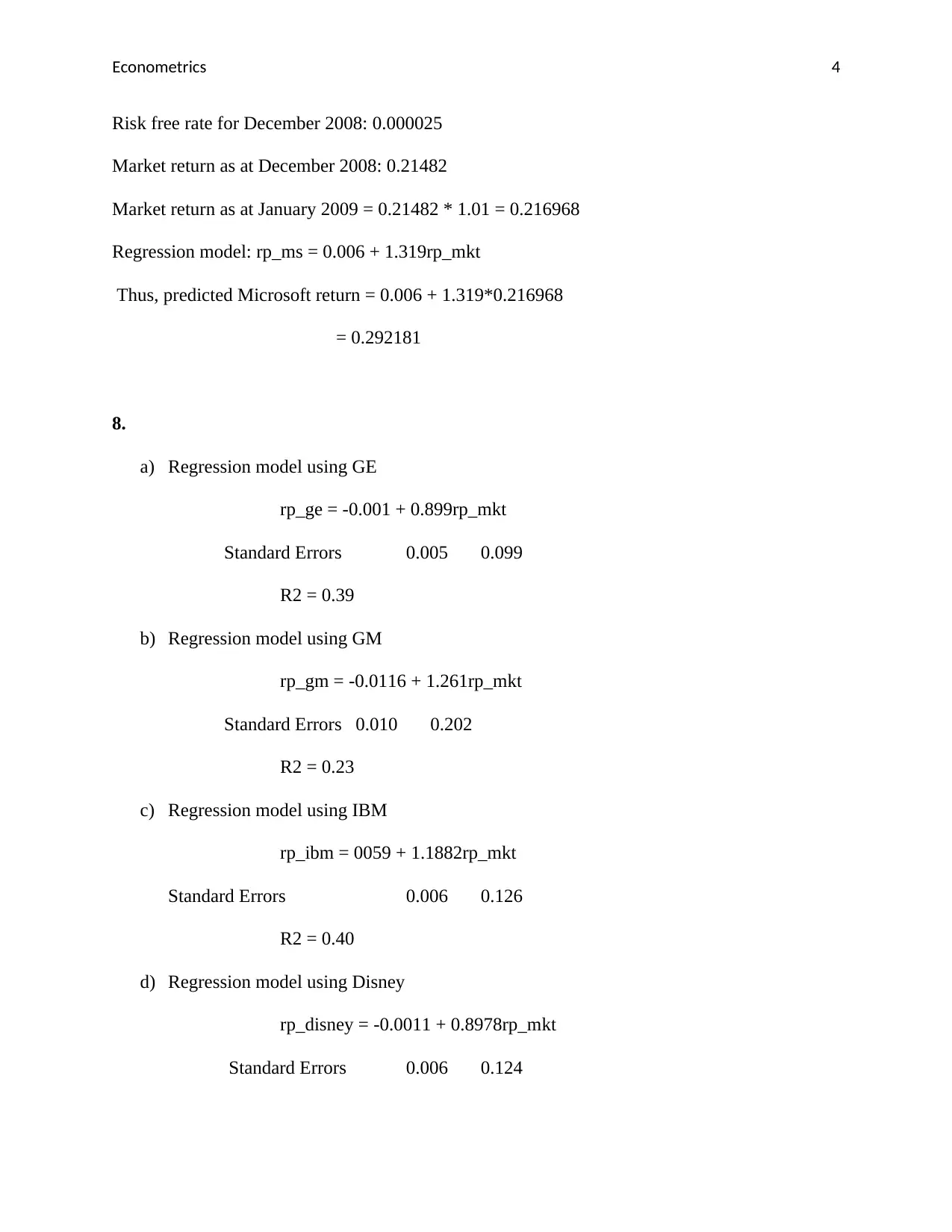
Homework Assignment
AI Summary
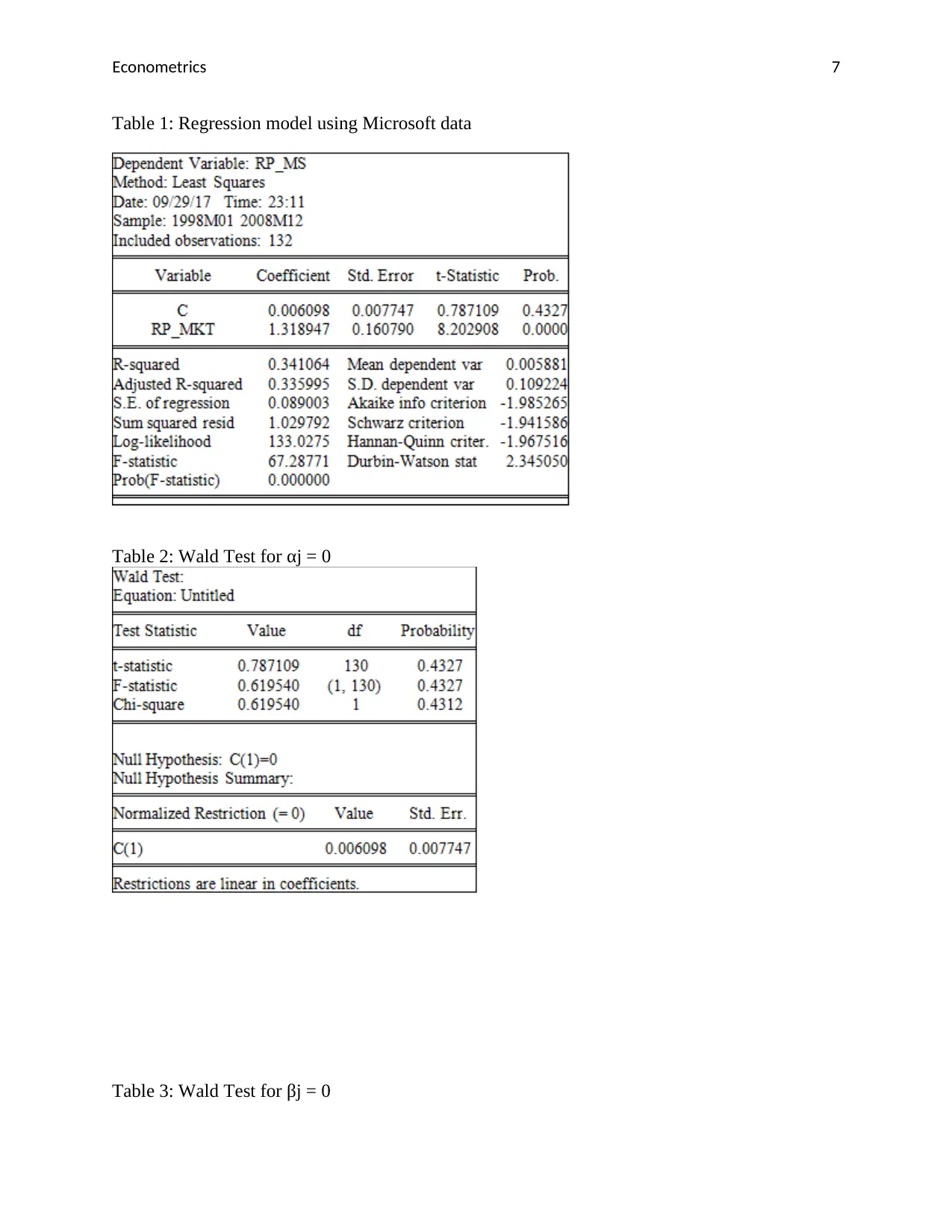
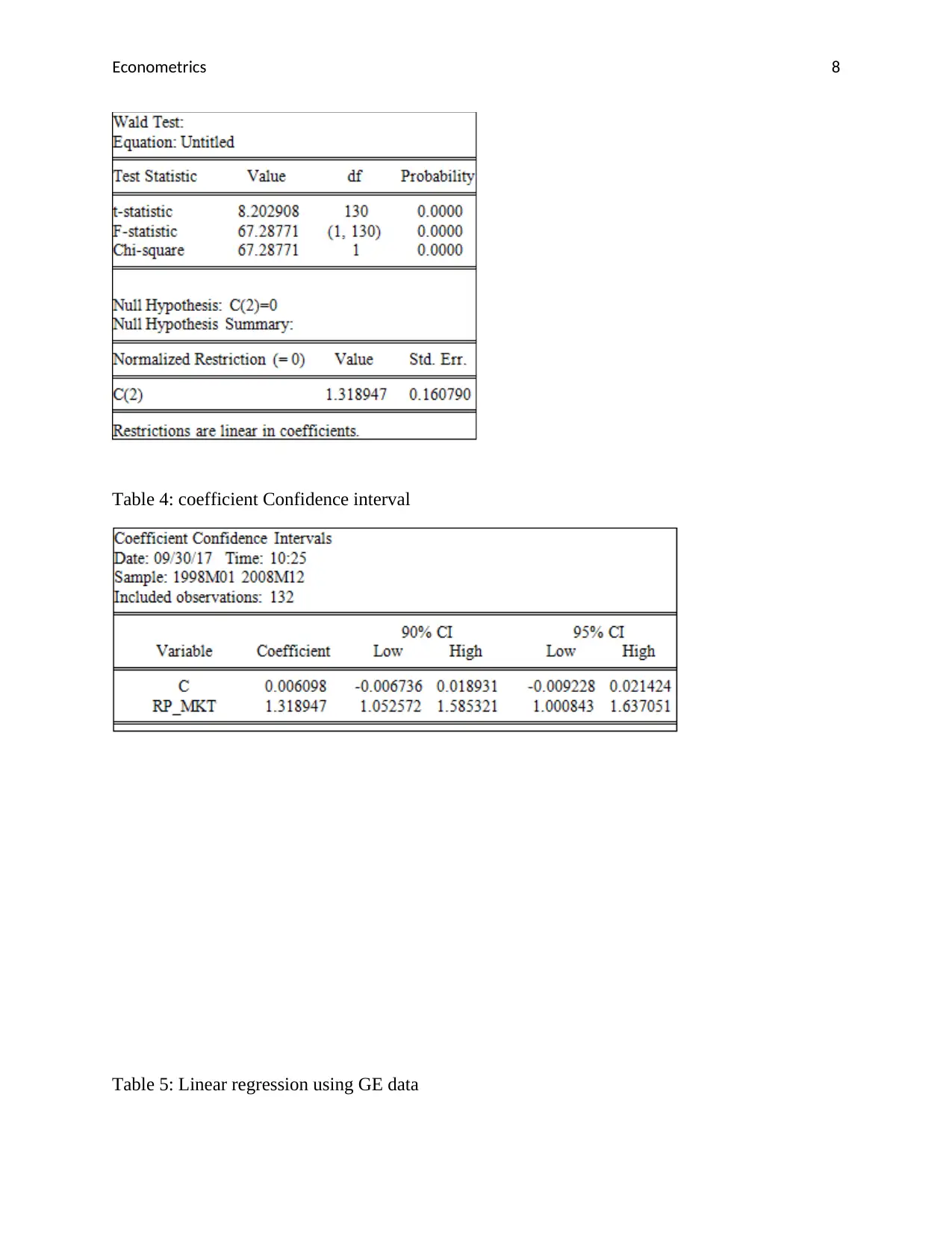
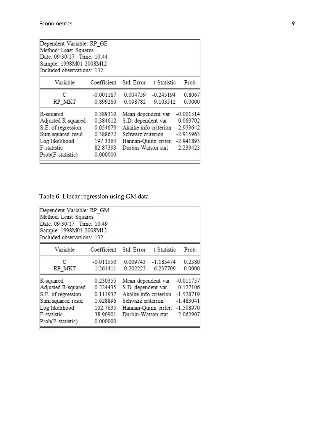
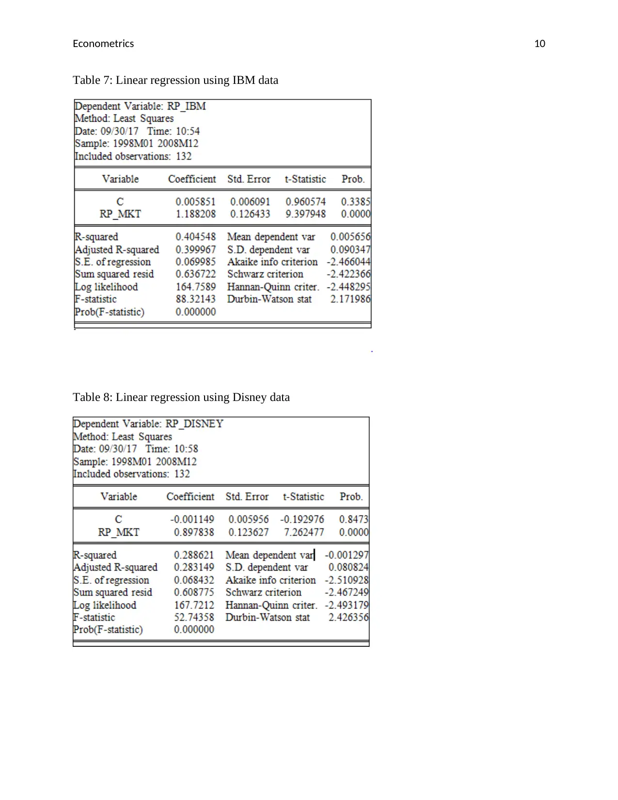
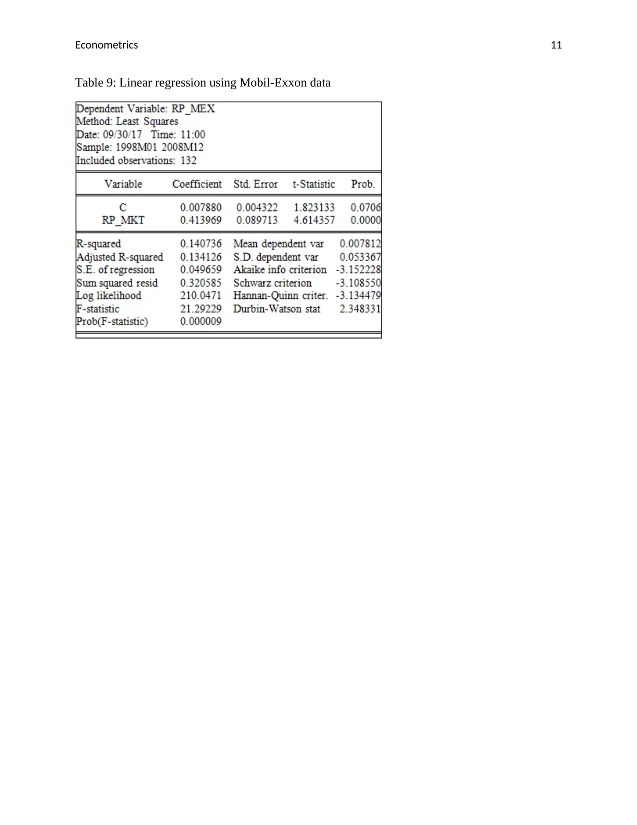
This econometrics assignment presents a regression analysis using Microsoft data, exploring concepts such as risk premium and beta values. The analysis includes the development and testing of hypotheses using Wald tests to determine the significance of coefficients. The assignment also calculates and interprets R-squared values, assesses confidence intervals for beta values, and predicts Microsoft's return based on market returns. Furthermore, it extends the analysis to include regression models for other companies like GE, GM, IBM, Disney, and Mobil-Exxon, providing a comparative view of their market behavior. The solution also includes several tables which provides detailed results of the analysis.
1 out of 11
Related Documents


Your All-in-One AI-Powered Toolkit for Academic Success.
+13062052269
info@desklib.com
Available 24*7 on WhatsApp / Email
![[object Object]](/_next/static/media/star-bottom.7253800d.svg)
Copyright © 2020–2026 A2Z Services. All Rights Reserved. Developed and managed by ZUCOL.