Econometrics Homework: CEO Salary and Wage Equation Analysis

This document presents a comprehensive solution to an econometrics homework assignment. It begins with theoretical exercises focusing on causality and its measurement, specifically addressing the impact of illegal downloads on subscription growth and evaluating the effect of 'ros' on CEO salary. The solution then delves into STATA exercises using the 'ceosal1.dta' dataset to model CEO salary determinants, calculate elasticity, and test hypotheses regarding the elasticity of salary with respect to sales. Further analysis employs the 'wage2.dta' dataset to interpret wage equation coefficients, assess their statistical significance, and test hypotheses about the impact of general work experience and tenure on wages, including constructing and interpreting a 95% confidence interval. The document provides detailed interpretations and statistical tests, demonstrating a strong understanding of econometric principles.

Econometrics
Student Name:
Instructor Name:
Course Number:
7th June 2019

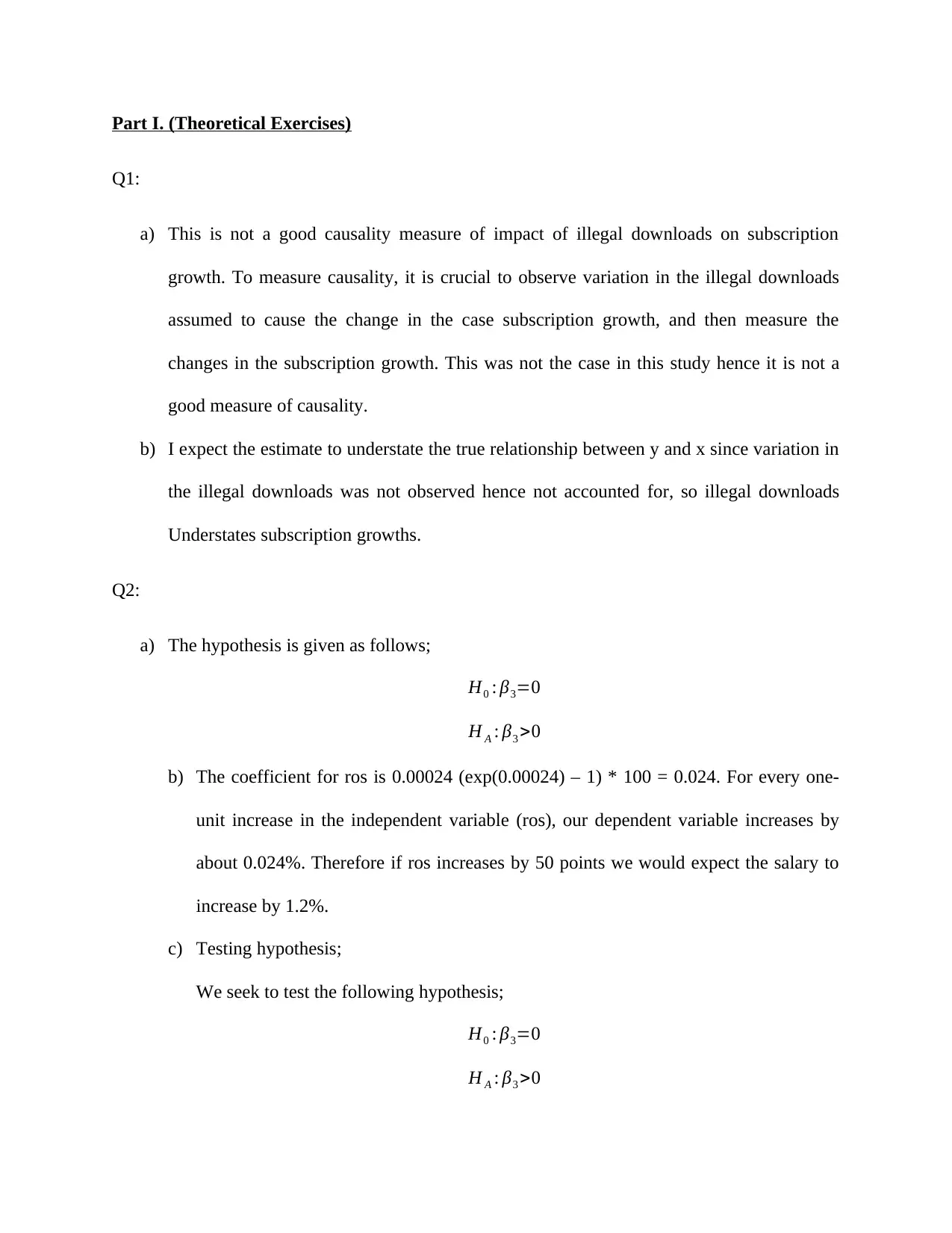
Part I. (Theoretical Exercises)
Q1:
a) This is not a good causality measure of impact of illegal downloads on subscription
growth. To measure causality, it is crucial to observe variation in the illegal downloads
assumed to cause the change in the case subscription growth, and then measure the
changes in the subscription growth. This was not the case in this study hence it is not a
good measure of causality.
b) I expect the estimate to understate the true relationship between y and x since variation in
the illegal downloads was not observed hence not accounted for, so illegal downloads
Understates subscription growths.
Q2:
a) The hypothesis is given as follows;
H0 : β3=0
H A : β3 >0
b) The coefficient for ros is 0.00024 (exp(0.00024) – 1) * 100 = 0.024. For every one-
unit increase in the independent variable (ros), our dependent variable increases by
about 0.024%. Therefore if ros increases by 50 points we would expect the salary to
increase by 1.2%.
c) Testing hypothesis;
We seek to test the following hypothesis;
H0 : β3=0
H A : β3 >0

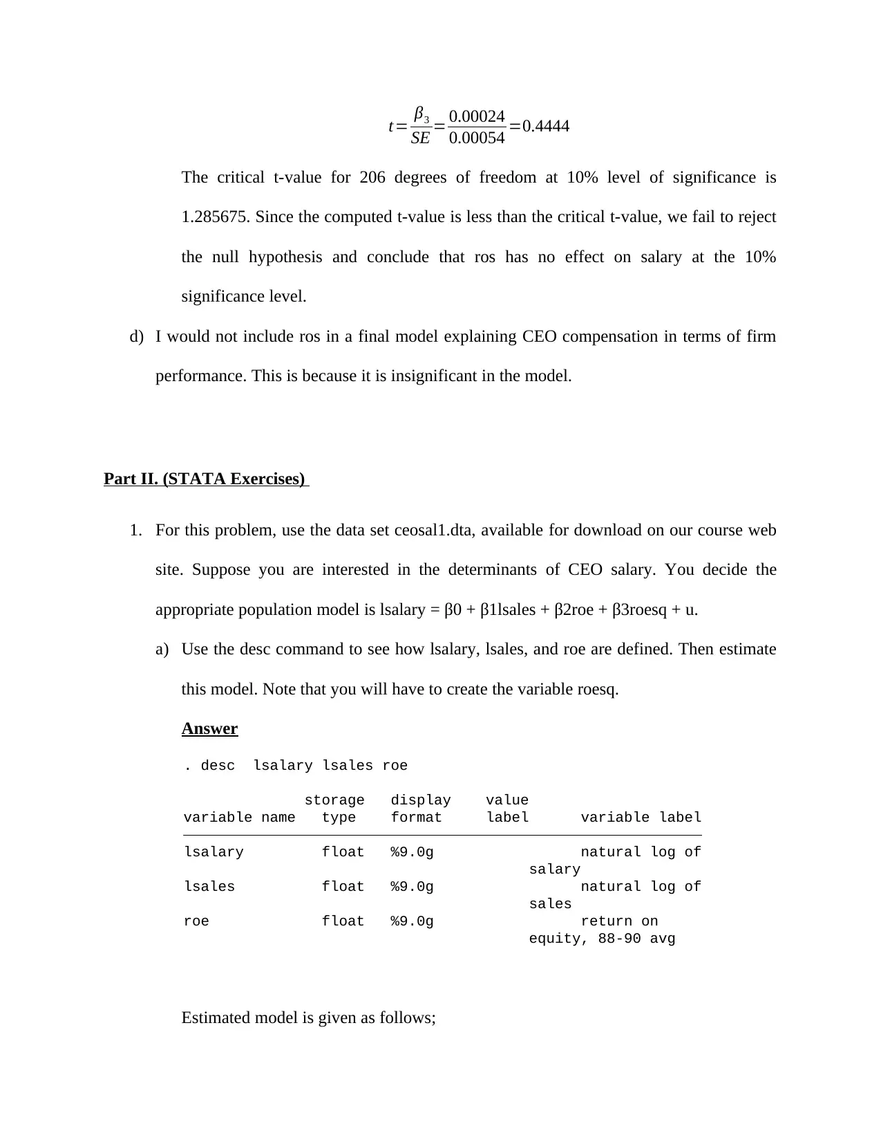
t= β3
SE = 0.00024
0.00054 =0.4444
The critical t-value for 206 degrees of freedom at 10% level of significance is
1.285675. Since the computed t-value is less than the critical t-value, we fail to reject
the null hypothesis and conclude that ros has no effect on salary at the 10%
significance level.
d) I would not include ros in a final model explaining CEO compensation in terms of firm
performance. This is because it is insignificant in the model.
Part II. (STATA Exercises)
1. For this problem, use the data set ceosal1.dta, available for download on our course web
site. Suppose you are interested in the determinants of CEO salary. You decide the
appropriate population model is lsalary = β0 + β1lsales + β2roe + β3roesq + u.
a) Use the desc command to see how lsalary, lsales, and roe are defined. Then estimate
this model. Note that you will have to create the variable roesq.
Answer
equity, 88-90 avg
roe float %9.0g return on
sales
lsales float %9.0g natural log of
salary
lsalary float %9.0g natural log of
variable name type format label variable label
storage display value
. desc lsalary lsales roe
Estimated model is given as follows;

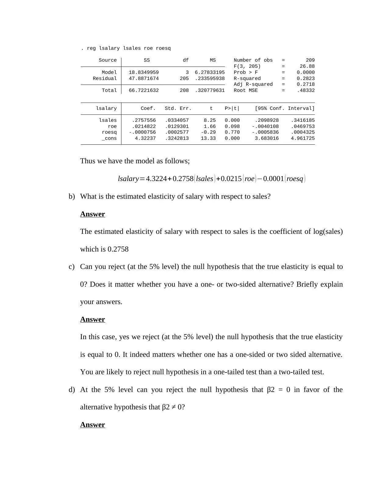
_cons 4.32237 .3242813 13.33 0.000 3.683016 4.961725
roesq -.0000756 .0002577 -0.29 0.770 -.0005836 .0004325
roe .0214822 .0129301 1.66 0.098 -.0040108 .0469753
lsales .2757556 .0334057 8.25 0.000 .2098928 .3416185
lsalary Coef. Std. Err. t P>|t| [95% Conf. Interval]
Total 66.7221632 208 .320779631 Root MSE = .48332
Adj R-squared = 0.2718
Residual 47.8871674 205 .233595938 R-squared = 0.2823
Model 18.8349959 3 6.27833195 Prob > F = 0.0000
F(3, 205) = 26.88
Source SS df MS Number of obs = 209
. reg lsalary lsales roe roesq
Thus we have the model as follows;
lsalary=4.3224+0.2758 ( lsales ) +0.0215 ( roe ) −0.0001 ( roesq )
b) What is the estimated elasticity of salary with respect to sales?
Answer
The estimated elasticity of salary with respect to sales is the coefficient of log(sales)
which is 0.2758
c) Can you reject (at the 5% level) the null hypothesis that the true elasticity is equal to
0? Does it matter whether you have a one- or two-sided alternative? Briefly explain
your answers.
Answer
In this case, yes we reject (at the 5% level) the null hypothesis that the true elasticity
is equal to 0. It indeed matters whether one has a one-sided or two sided alternative.
You are likely to reject null hypothesis in a one-tailed test than a two-tailed test.
d) At the 5% level can you reject the null hypothesis that β2 = 0 in favor of the
alternative hypothesis that β2 ≠ 0?
Answer

The p-value for the coefficient β2 is 0.098 (a value greater than 5% level) hence we
fail to reject the null hypothesis that β2 = 0 in favor of the alternative hypothesis that
β2 ≠ 0.
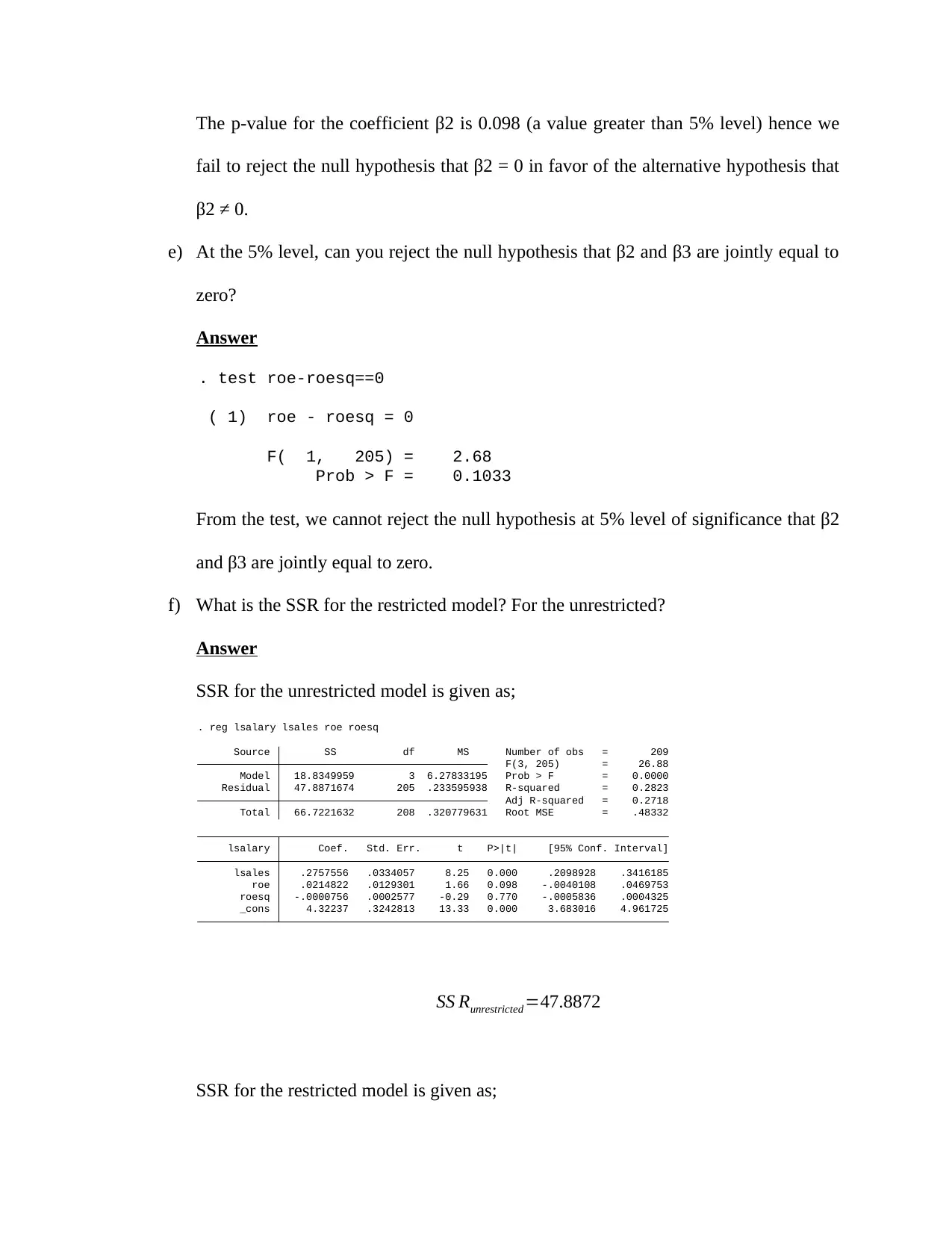
e) At the 5% level, can you reject the null hypothesis that β2 and β3 are jointly equal to
zero?
Answer
Prob > F = 0.1033
F( 1, 205) = 2.68
( 1) roe - roesq = 0
. test roe-roesq==0
From the test, we cannot reject the null hypothesis at 5% level of significance that β2
and β3 are jointly equal to zero.
f) What is the SSR for the restricted model? For the unrestricted?
Answer
SSR for the unrestricted model is given as;
_cons 4.32237 .3242813 13.33 0.000 3.683016 4.961725
roesq -.0000756 .0002577 -0.29 0.770 -.0005836 .0004325
roe .0214822 .0129301 1.66 0.098 -.0040108 .0469753
lsales .2757556 .0334057 8.25 0.000 .2098928 .3416185
lsalary Coef. Std. Err. t P>|t| [95% Conf. Interval]
Total 66.7221632 208 .320779631 Root MSE = .48332
Adj R-squared = 0.2718
Residual 47.8871674 205 .233595938 R-squared = 0.2823
Model 18.8349959 3 6.27833195 Prob > F = 0.0000
F(3, 205) = 26.88
Source SS df MS Number of obs = 209
. reg lsalary lsales roe roesq
SS Runrestricted =47.8872
SSR for the restricted model is given as;

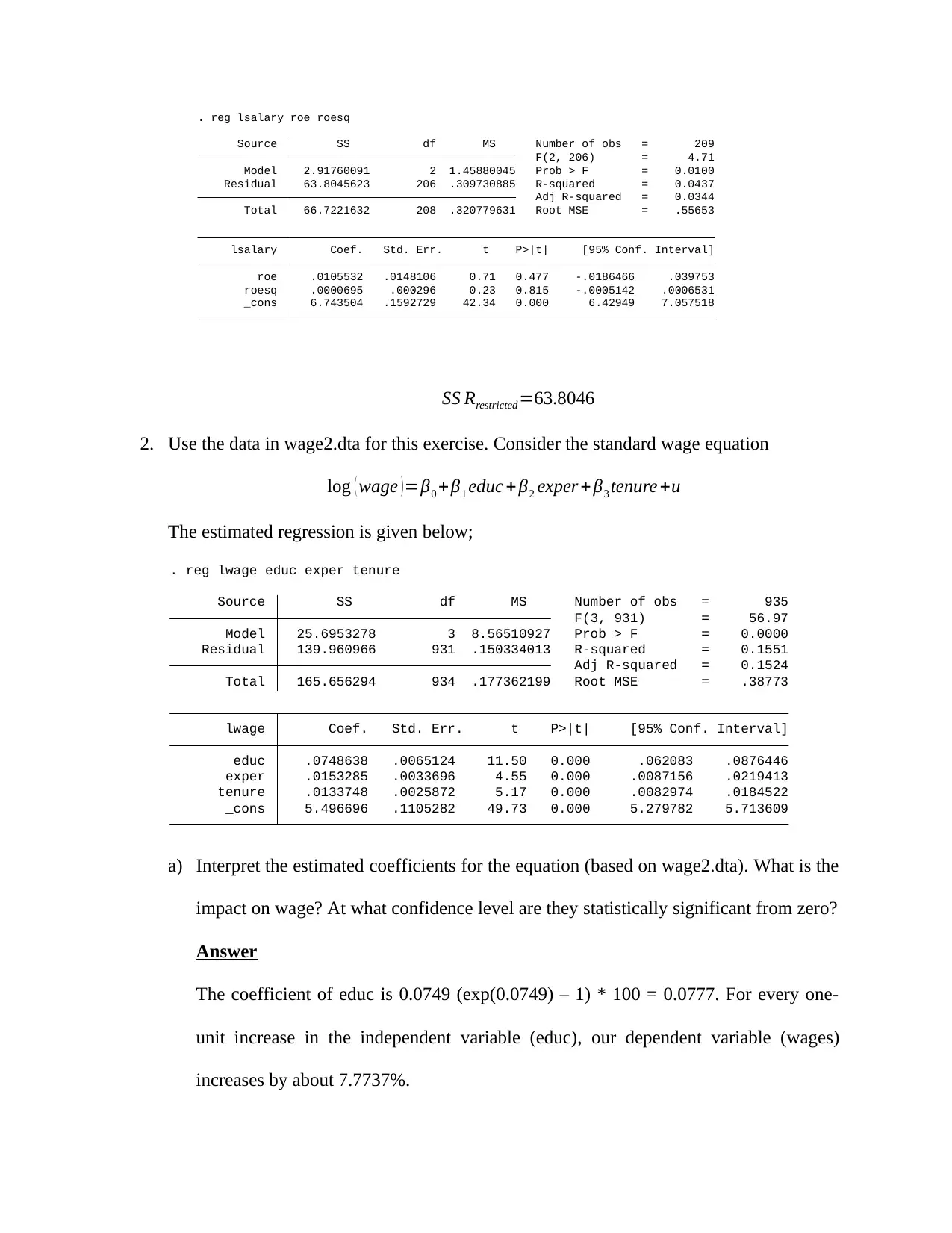
_cons 6.743504 .1592729 42.34 0.000 6.42949 7.057518
roesq .0000695 .000296 0.23 0.815 -.0005142 .0006531
roe .0105532 .0148106 0.71 0.477 -.0186466 .039753
lsalary Coef. Std. Err. t P>|t| [95% Conf. Interval]
Total 66.7221632 208 .320779631 Root MSE = .55653
Adj R-squared = 0.0344
Residual 63.8045623 206 .309730885 R-squared = 0.0437
Model 2.91760091 2 1.45880045 Prob > F = 0.0100
F(2, 206) = 4.71
Source SS df MS Number of obs = 209
. reg lsalary roe roesq
SS Rrestricted=63.8046
2. Use the data in wage2.dta for this exercise. Consider the standard wage equation
log ( wage ) =β0 +β1 educ + β2 exper + β3 tenure +u
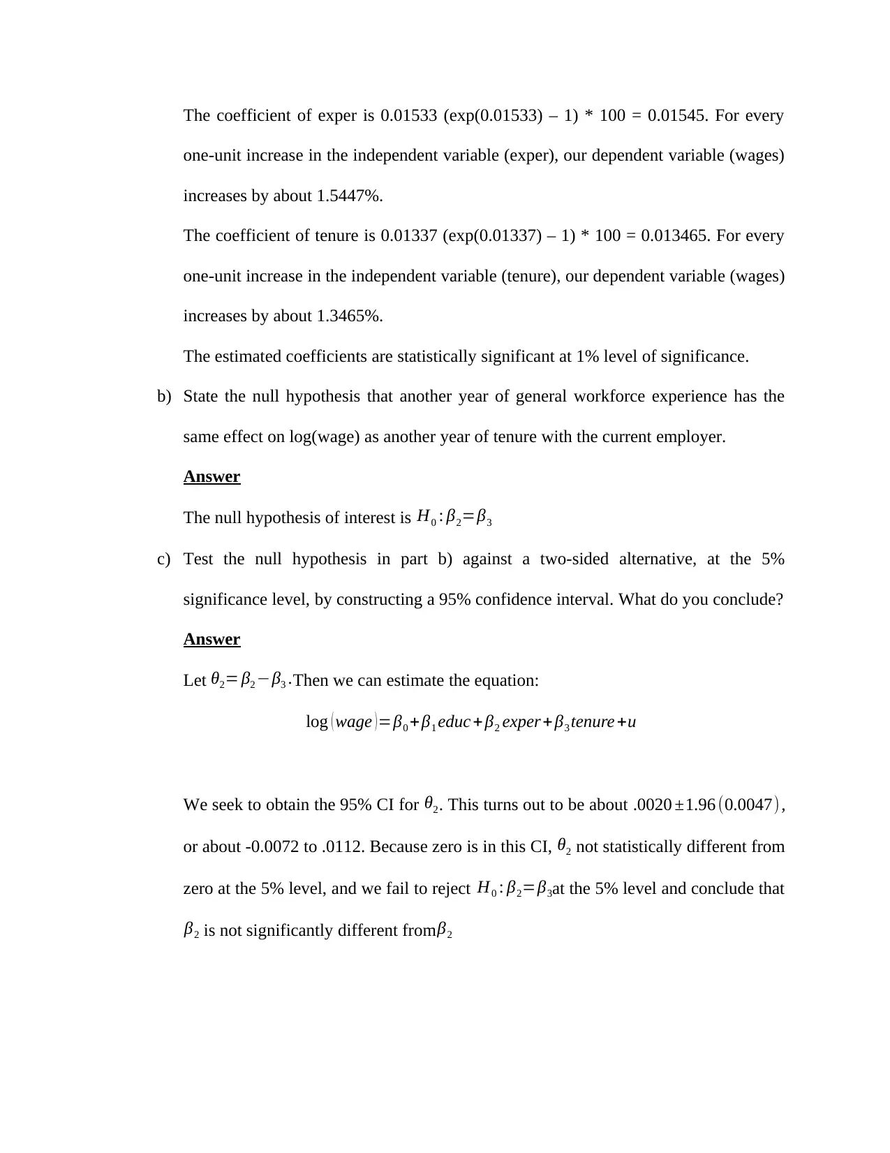
The estimated regression is given below;
_cons 5.496696 .1105282 49.73 0.000 5.279782 5.713609
tenure .0133748 .0025872 5.17 0.000 .0082974 .0184522
exper .0153285 .0033696 4.55 0.000 .0087156 .0219413
educ .0748638 .0065124 11.50 0.000 .062083 .0876446
lwage Coef. Std. Err. t P>|t| [95% Conf. Interval]
Total 165.656294 934 .177362199 Root MSE = .38773
Adj R-squared = 0.1524
Residual 139.960966 931 .150334013 R-squared = 0.1551
Model 25.6953278 3 8.56510927 Prob > F = 0.0000
F(3, 931) = 56.97
Source SS df MS Number of obs = 935
. reg lwage educ exper tenure
a) Interpret the estimated coefficients for the equation (based on wage2.dta). What is the
impact on wage? At what confidence level are they statistically significant from zero?
Answer
The coefficient of educ is 0.0749 (exp(0.0749) – 1) * 100 = 0.0777. For every one-
unit increase in the independent variable (educ), our dependent variable (wages)
increases by about 7.7737%.

The coefficient of exper is 0.01533 (exp(0.01533) – 1) * 100 = 0.01545. For every
one-unit increase in the independent variable (exper), our dependent variable (wages)
increases by about 1.5447%.
The coefficient of tenure is 0.01337 (exp(0.01337) – 1) * 100 = 0.013465. For every
one-unit increase in the independent variable (tenure), our dependent variable (wages)
increases by about 1.3465%.
The estimated coefficients are statistically significant at 1% level of significance.
b) State the null hypothesis that another year of general workforce experience has the
same effect on log(wage) as another year of tenure with the current employer.
Answer
The null hypothesis of interest is H0 : β2=β3
c) Test the null hypothesis in part b) against a two-sided alternative, at the 5%
significance level, by constructing a 95% confidence interval. What do you conclude?
Answer
Let θ2= β2 −β3 .Then we can estimate the equation:
log ( wage )=β0 +β1 educ + β2 exper+ β3 tenure +u
We seek to obtain the 95% CI for θ2. This turns out to be about .0020 ±1.96 (0.0047) ,
or about -0.0072 to .0112. Because zero is in this CI, θ2 not statistically different from
zero at the 5% level, and we fail to reject H0 : β2=β3at the 5% level and conclude that
β2 is not significantly different from β2