Econometrics Assignment: Regression Analysis and Testing
VerifiedAdded on 2020/02/05
|9
|1006
|254
Homework Assignment
AI Summary
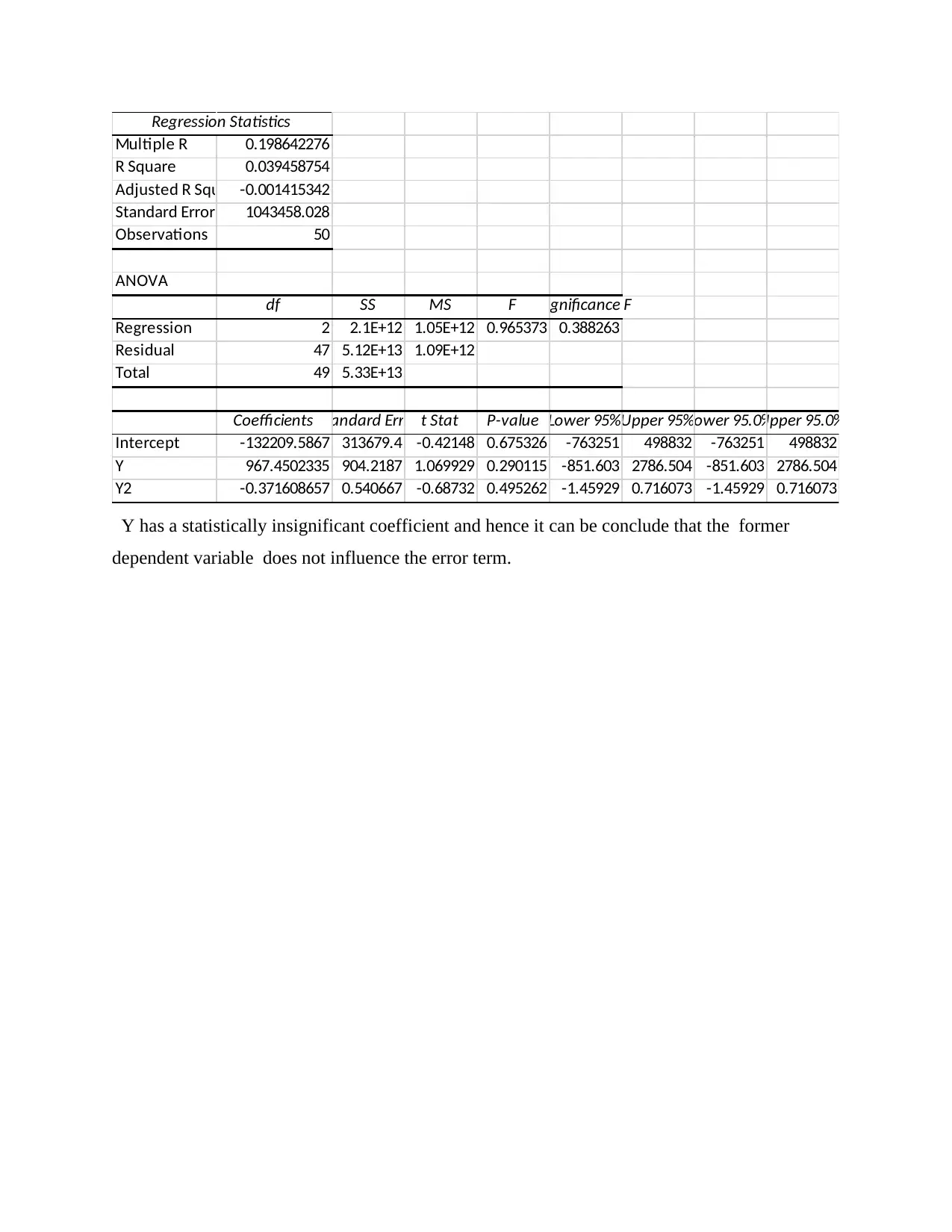
This document provides a comprehensive solution to an econometrics assignment. It delves into the analysis of two economic models. The first model explores factors influencing beer consumption, including price, price of other liquor, and income, using OLS regression, hypothesis testing (F-test, t-test), and tests for model specification (RESET) and multicollinearity. It examines the significance of coefficients and the overall model. The second model investigates factors affecting oil consumption, such as the number of registered vehicles and taxation, also employing regression analysis and hypothesis testing. It tests for heteroscedasticity (Goldfeld-Quandt Test, White test), normality of errors, and model specification (RESET). The solution interprets the regression coefficients, conducts statistical tests, and assesses the validity and robustness of each model.

a. Given
Qt =α PBt
β 2 PLt
β 3 PRt
β 4 It
β 5 exp {et }∧et N (0 , σ2 )
The model may be rewritten in linear form (by applying logs) as:
logQt =log α + β2 log PBt + β3 log PLt + β4 log PRt + β5 log It +log et
Using the data provided, the log-log linear model is estimated using OLS as;
SUMMARY OUTPUT
Regression Statistics
Multiple R 0.908508994
R Square 0.825388591
Adjusted R Square0.797450766
Standard Error 0.026046069
Observations 30
ANOVA
df SS MS F Significance F
Regression 4 0.080169692 0.020042 29.54377 3.8E-09
Residual 25 0.016959942 0.000678
Total 29 0.097129635
Coefficients Standard Error t Stat P-value Lower 95%Upper 95%Lower 95.0%Upper 95.0%
Intercept -1.40852023 1.625564037 -0.86648 0.394467 -4.75643 1.939392 -4.75643 1.939392
Log PB -1.02041877 0.23904185 -4.26879 0.000248 -1.51273 -0.5281 -1.51273 -0.5281
Log PL -0.58293365 0.560150059 -1.04067 0.307987 -1.73658 0.570717 -1.73658 0.570717
log PR 0.209544972 0.079692634 2.629415 0.014422 0.045415 0.373675 0.045415 0.373675
Log I 0.922863752 0.415514182 2.221016 0.035639 0.067096 1.778631 0.067096 1.778631
logQt =log−1.4085−1.0204 log PBt−0.5829 log PLt +0.2095 log PRt + 0.9229 log I t
SE1.6255 0.2390 0.5602 0.07969 0.4155
b. Interpreted the regression coefficients
From the estimated model α = -1.4085, implying that the average quantity of beer consumed
is negative, if all other factors include in the model remain at zero. But then again the value is
not statistically significant it has a p-value of 0.39 which is larger than the significance level
(0.05)
Holding other factors constant, a 100 % rise in the price of beer would reduce beer
consumption by 102.04% and vice versa. The value is statistically different from zero.
Consequently, ceteris paribus a 100% change in PR and income would change alcohol
consumption by 20.95% and 92.28% respectively. These values are also statistically
Paraphrase This Document
Need a fresh take? Get an instant paraphrase of this document with our AI Paraphraser

significant. Note that β3 has p-value larger than significant level and hence has its estimated
value does not have statistical significance. However, the negative sign implies that a rise in
price liquor ma lead to a reduction in beer consumption.
c. Overall significance
From t the output table, the significance F = 0.0000000038 which is less than the
significance level (0.05), hence at least of non-constant coefficients is not zero and hence
the model is significant at 95% confidence level.
d. Test the hypothesis H0= β3 =β4=0 against H A =either β3∨β4∨bothare not zero
If the β3=β4 =0 then the model would reduce from
logQt =log α + β2 log PBt + β3 log PLt + β4 log PRt + β5 log I t + log et … … … … …..(UR )
To
logQt =log α +β2 log PBt + β5 log I t +log et … … … … … … … … … … . Restricted model(R)
Table 2(restricted model)
SUMMARY OUTPUT
Regression Statistics
Multiple R 0.88017
R Square 0.774699
Adjusted R Square0.75801
Standard Error0.028469
Observations 30
ANOVA
df SS MS F Significance F
Regression 2 0.075246 0.037623 46.41988 1.83E-09
Residual 27 0.021883 0.00081
Total 29 0.09713
CoefficientsStandard Error t Stat P-value Lower 95%Upper 95%Lower 95.0%Upper 95.0%
Intercept -2.90242 1.527086 -1.90062 0.068077 -6.03574 0.230905 -6.03574 0.230905
Log I 1.160386 0.362463 3.201392 0.003487 0.416673 1.904098 0.416673 1.904098
Log PB -1.22125 0.231322 -5.27942 1.44E-05 -1.69588 -0.74661 -1.69588 -0.74661
Using the F –test

F statistic=
( RUR
2 −RR
2 )
q
(1−RUR
2 )
( n−k )
Where n = number of observation = 30
k = is the degrees of freedom = 4
q= number of restrictions = 2
R2UR is the R-Squared of the unrestricted model = 0.8254 (from table 1)
R2R is the R-Squared of the restricted model = 0.7746 (from table 2)
F statistic=
0.8254−0.7746
2
( 1−0.8254
30−4 ) =3.7824
F critical
F2, 26
0.05 =3.3690
The F statistic is greater than the critical F, and hence the hypothesis is rejected, implying that
both β3∧β4 cannot be statistically equal to zero. At least one of the two is not zero, and hence
the unrestricted model is better than the restricted model.
e. Test the hypothesis H0 : β2+ β3 + β4 =β5 =0 against HA: at least one of the coefficients is not
zero
If the β2+ β3 +β4 =β5=0 then the model would reduce to
logQt =log α
And q =k = 4
The f value
Fvalue=
R2
k
( 1−R2 )
( n−k )
=
0.8254
4
( 1−0.8254
30−4 )=30.72
Note that the F calculated value may also be obtained from table 1 (F ≈ 29.54376).
F critical
F2, 26
0.05 =3.3690
⊘ This is a preview!⊘
Do you want full access?
Subscribe today to unlock all pages.

Trusted by 1+ million students worldwide

Notably, calculated F is greater than the critical F, and hence the null hypothesis is rejected. The
implication is that at least one of the coefficients is statistically different from zero and hence the
model is better than the constant model.
f. Test whether beer and other liquor are competing products (β3 is negative)
H0: β3 = 0
HA: β3 < 0
Using the t-statistics
tcalculated = β3
SE = 0.582933645
0.560150059 =1.040674077
T critical
t0.05 ,28=1.701
The t static in this case is smaller than the critical t value, and hence the null hypothesis is not
rejected. Therefore, in accordance with this sample, beer and other liquor are not competing
products, in the senses that the quantity of beer consumed is not influenced by changes in other
liquor’s prices.
g. Error term is normally distributed
From the above Normal probability plot, the error term appears to be normally
distributed, as all but one value tends to form a straight line.
h. Using RESET to tests the model significance
Assume a different model:
logQt =log α +β2 log PBt + β3 log PLt + β4 log PRt + β5 log It +(logQ¿¿ t)3 +log et ¿
Paraphrase This Document
Need a fresh take? Get an instant paraphrase of this document with our AI Paraphraser

SUMMARY OUTPUT
Regression Statistics
Multiple R 0.999328
R Square 0.998657
Adjusted R Square0.998377
Standard Error0.002331
Observations 30
ANOVA
df SS MS F Significance F
Regression 5 0.096999 0.0194 3568.902 1.25E-33
Residual 24 0.00013 5.44E-06
Total 29 0.09713
CoefficientsStandard Error t Stat P-value Lower 95%Upper 95%Lower 95.0%Upper 95.0%
Intercept 1.450216 0.154314 9.397818 1.63E-09 1.131727 1.768705 1.131727 1.768705
Log PB 0.094882 0.029319 3.236169 0.003518 0.03437 0.155394 0.03437 0.155394
Log PL 0.005261 0.051243 0.102664 0.919082 -0.1005 0.111022 -0.1005 0.111022
log PR -0.02266 0.008265 -2.74198 0.011356 -0.03972 -0.0056 -0.03972 -0.0056
Log I -0.07835 0.041318 -1.89631 0.07002 -0.16363 0.006924 -0.16363 0.006924
(log Q)3 0.112505 0.002022 55.64212 6.94E-27 0.108332 0.116678 0.108332 0.116678
The extra variable has a coefficient which is statistically different from zero (p-value is less than
0.05), and hence there is a misspecification. The model is not adequate at 5% significance level.
i. Multicolinearity
Correlation
Log PB Log PL log PR Log I
Log PB 1
Log PL 0.966883 1
log PR 0.77393 0.809413 1
Log I 0.971055 0.97146 0.821124 1
Some of the explanatory variables show a very strong correlation, suggesting a possible
existence of multicollinearity. The price of beer, price of other liquor and income show strong
correlation.

Question 2
a. Given the model
PCON i=β1 + β2 REGi +β3 TAXi +ei
The model is estimated as:
SUMMARY OUTPUT
Regression Statistics
Multiple R 0.687811
R Square 0.473084
Adjusted R Square0.450662
Standard Error502.3873
Observations 50
ANOVA
df SS MS F Significance F
Regression 2 10650532 5325266 21.09911 2.89E-07
Residual 47 11862469 252393
Total 49 22513001
CoefficientsStandard Error t Stat P-value Lower 95%Upper 95%Lower 95.0%Upper 95.0%
Intercept 1158.438 355.9405 3.254584 0.002108 442.3784 1874.498 442.3784 1874.498
REG 0.173512 0.032277 5.375696 2.34E-06 0.108579 0.238445 0.108579 0.238445
TAX -102.844 32.60363 -3.15438 0.002803 -168.434 -37.2542 -168.434 -37.2542
PCONi=1158.438+0.1735 REGi −102.844 TAXi
All the estimates are statistically significant at 95% confidence level. The intercept β1 implies
that on average each state consumes 1158.438 million of BTU. Holding taxation constant, a unit
increase in the number of registered vehicles increases oil consumption by 0.1735 million BTU,
a change in tax by one cent per gallon, reduces oil consumption by 102.844 if all other factors in
the model do not change.
b. Construct and interpret the 95% confidence interval for β3
Using the t –test, the hypothesis is formulated as
H0 : β3=0
H A : β3 ≠ 0
Since he p-value ( from the table) is less than 0.05, the null hypothesis is rejected implying β3 is
statistically not zero and hence tax impacts oil consumption.
⊘ This is a preview!⊘
Do you want full access?
Subscribe today to unlock all pages.

Trusted by 1+ million students worldwide

c. Goldfeld-Quandt Test
The hypothesis is set as;
H0 :σ1=σ2 …=σk=0
H1 : at least one of the variances ∈HO is not zero
F= RSSupper
RSSlower
= 2459384.551
28955.93725 =84.935
F-critical
F15, 15
0.05 =2.4034
The F calculated value is larger than the critical F and hence the null hypothesis is rejected.
The model is not homoscedastic (heteroscedasticity is present).
d.
The hypothesis is set as;
H0 :σ1=σ2 …=σk=0
H1 : at least one of the variances ∈HO is not zero
F= RSSupper
RSSlower
= 59450.50796
5319348.461 =0.011176276
F-critical
F15, 15
0.05 =2.4034
The F calculated value is less than the critical F and hence the null hypothesis is not rejected.
The model is homoscedastic (heteroscedasticity is not present).
e. Normality in error terms
0 20 40 60 80 100 120
0
1000
2000
3000
4000
Normal Probability Plot
Sample Percentile
PCON
The hypothesis is set as;
H0 :σ1=σ2 …=σk=0
H1 : at least one of the variances ∈HO is not zero
F= RSSupper
RSSlower
= 2459384.551
28955.93725 =84.935
F-critical
F15, 15
0.05 =2.4034
The F calculated value is larger than the critical F and hence the null hypothesis is rejected.
The model is not homoscedastic (heteroscedasticity is present).
d.
The hypothesis is set as;
H0 :σ1=σ2 …=σk=0
H1 : at least one of the variances ∈HO is not zero
F= RSSupper
RSSlower
= 59450.50796
5319348.461 =0.011176276
F-critical
F15, 15
0.05 =2.4034
The F calculated value is less than the critical F and hence the null hypothesis is not rejected.
The model is homoscedastic (heteroscedasticity is not present).
e. Normality in error terms
0 20 40 60 80 100 120
0
1000
2000
3000
4000
Normal Probability Plot
Sample Percentile
PCON
Paraphrase This Document
Need a fresh take? Get an instant paraphrase of this document with our AI Paraphraser

The Normal probability plot does not assume a straight line and hence errors are not
normally distributed.
f. RESET test
Assume the model was specified as
PCONi=β1 +β2 REGi +β3 TAXi + β4 PCONi
2+ei
The hypothesis to be tested is whether β4 is statistically significant.
SUMMARY OUTPUT
Regression Statistics
Multiple R 0.990948
R Square 0.981978
Adjusted R Square0.980802
Standard Error93.91635
Observations 50
ANOVA
df SS MS F Significance F
Regression 3 22107268 7369089 835.471 4.17E-40
Residual 46 405732.9 8820.281
Total 49 22513001
CoefficientsStandard Error t Stat P-value Lower 95%Upper 95%Lower 95.0%Upper 95.0%
Intercept 233.6454 71.31582 3.276208 0.002005 90.09414 377.1967 90.09414 377.1967
REG 0.104382 0.006331 16.48644 6.23E-21 0.091638 0.117127 0.091638 0.117127
TAX -12.8706 6.586388 -1.95412 0.056783 -26.1283 0.387133 -26.1283 0.387133
(PCON)2 0.000257 7.12E-06 36.04037 2.29E-35 0.000242 0.000271 0.000242 0.000271
With a p-value of 2.29 * 10-35, the squared value has a statistically significant coefficient and
hence the model was not adequately specified.
g. White test
Assume the model ^ε i
2=β1+β2 ^Y i+ β3 ^Y ii
2 + μi
Where ^ε i
2 are the squared residuals obtained from a
^Y i are the estimated values of PCON
μiis a set of disturbances?
The model is estimated as:

Regression Statistics
Multiple R 0.198642276
R Square 0.039458754
Adjusted R Square-0.001415342
Standard Error 1043458.028
Observations 50
ANOVA
df SS MS F Significance F
Regression 2 2.1E+12 1.05E+12 0.965373 0.388263
Residual 47 5.12E+13 1.09E+12
Total 49 5.33E+13
Coefficients Standard Error t Stat P-value Lower 95%Upper 95%Lower 95.0%Upper 95.0%
Intercept -132209.5867 313679.4 -0.42148 0.675326 -763251 498832 -763251 498832
Y 967.4502335 904.2187 1.069929 0.290115 -851.603 2786.504 -851.603 2786.504
Y2 -0.371608657 0.540667 -0.68732 0.495262 -1.45929 0.716073 -1.45929 0.716073
Y has a statistically insignificant coefficient and hence it can be conclude that the former
dependent variable does not influence the error term.
⊘ This is a preview!⊘
Do you want full access?
Subscribe today to unlock all pages.

Trusted by 1+ million students worldwide
1 out of 9