Econometrics Assignment: ADF Test on Traffic Accident Data

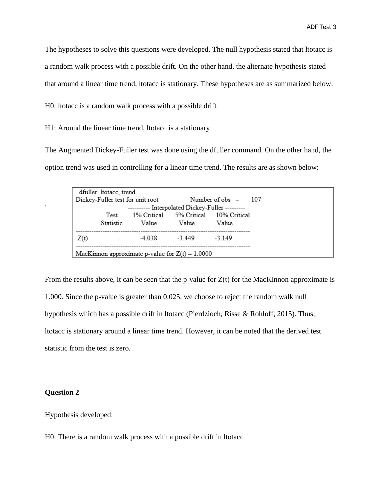
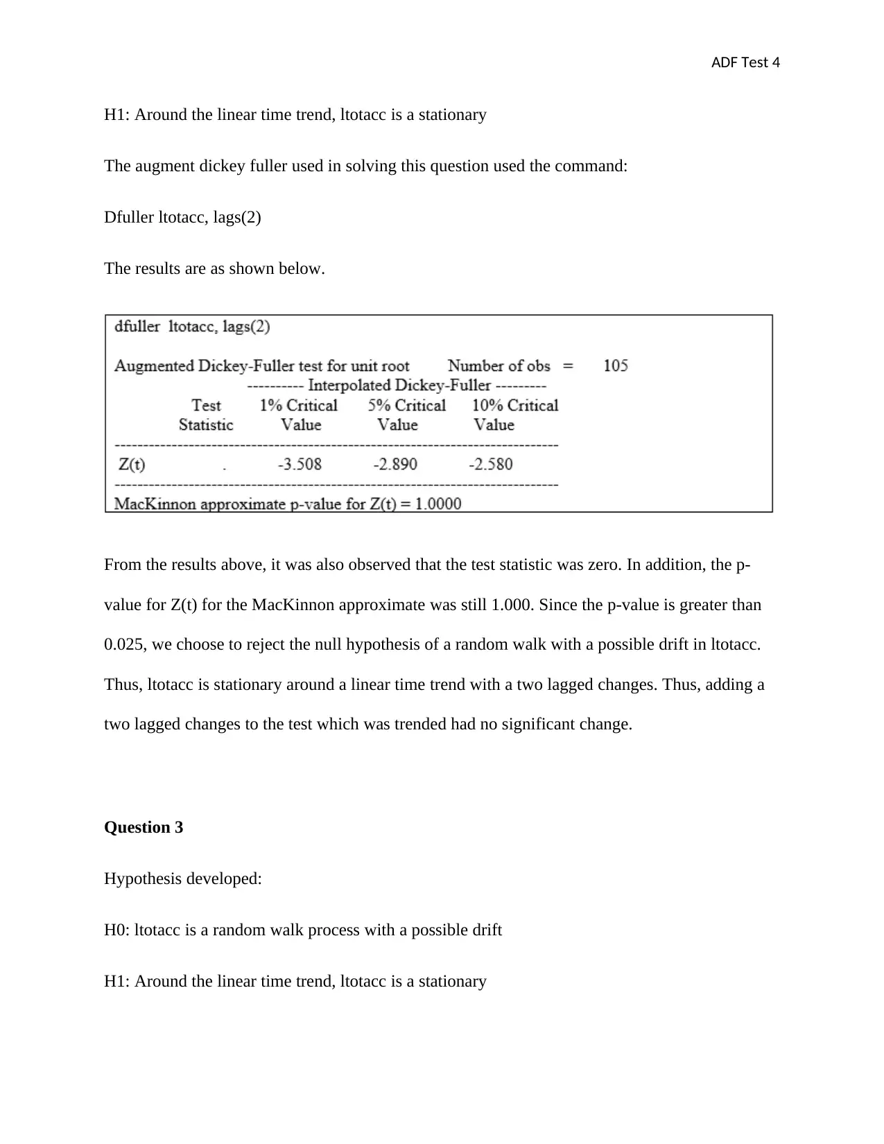
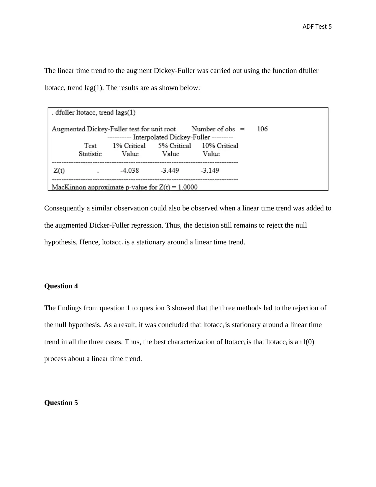
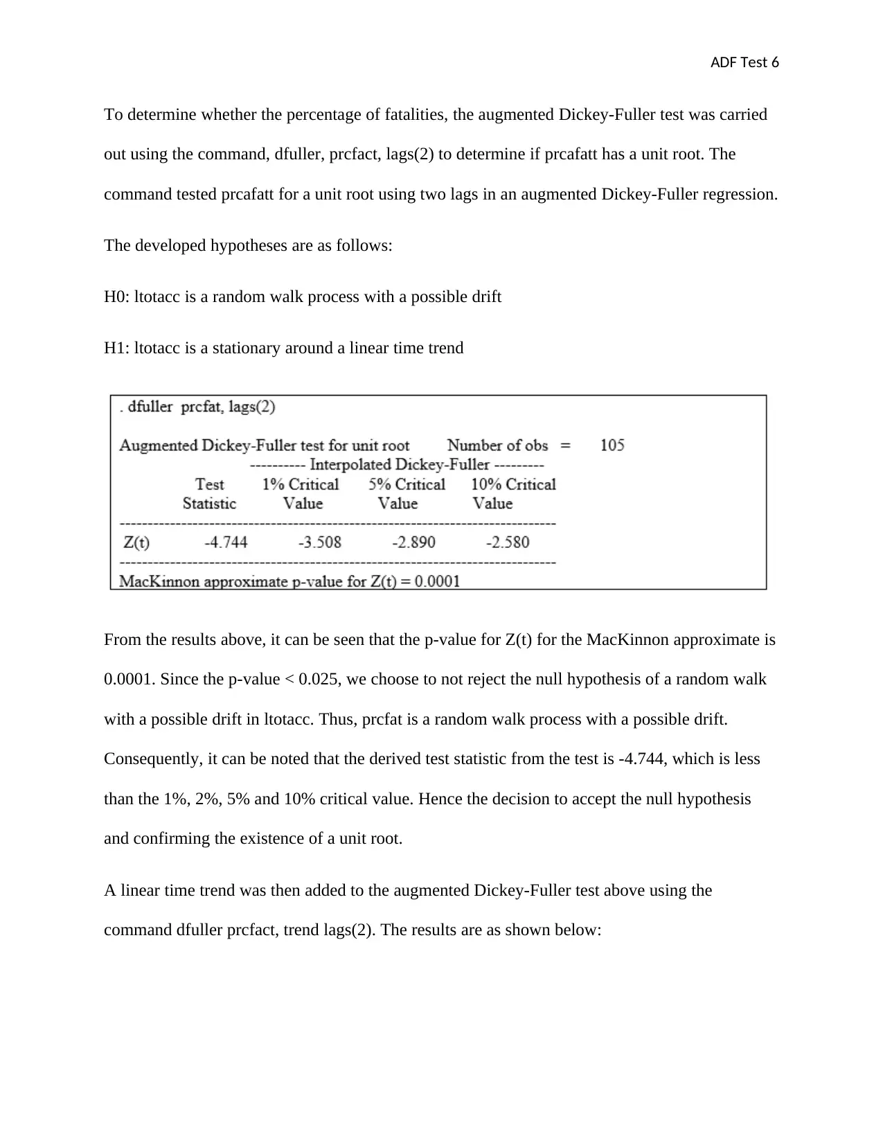
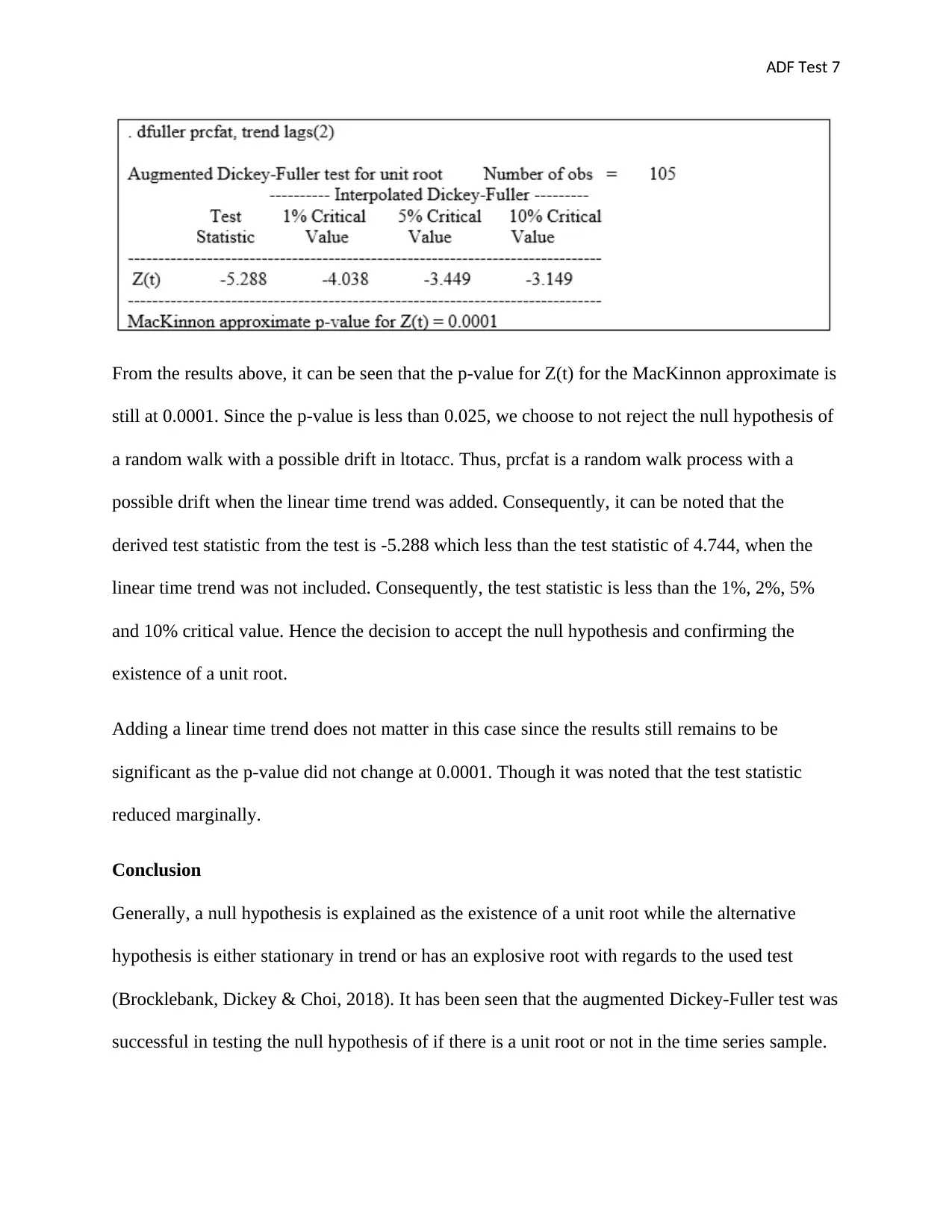
This assignment analyzes traffic accident data using the Augmented Dickey-Fuller (ADF) test to determine the presence of unit roots in time series variables. The analysis begins with a standard Dickey-Fuller regression on the log of total accidents (ltotacc) to test for a unit root, rejecting the null hypothesis and concluding stationarity around a linear time trend. Further analysis incorporates lagged changes and a linear time trend in the ADF regression, confirming the initial findings. The assignment then tests the percentage of fatalities (prcfatt) and finds evidence of a unit root, regardless of whether a linear time trend is included. The document concludes that ltotacc is best characterized as an I(0) process about a linear time trend, while prcfatt is a random walk process with a possible drift. The student employed the dfuller command in STATA to perform the ADF test.

ADF TEST 1
ADF Test
Student’s name:
Student’s ID:
Institution:

ADF Test 2
Introduction
The Dickey-Fuller test is employed in determining the presence of a unit root in an
autoregressive model (Paparoditis & Politis, 2018). The feature of a unit root can bring about
problems in statistical inference. Developed in 1979 by two statisticians of American origin,
David Dickey and Wayne Fuller, the formula is appropriate for time series trending (Ramenah et
al., 2018). The Dickey-Fuller test is the simplest approach in testing for a unit root. The test of an
augmented Dickey-Fuller comes into perspective since most financial and economic time series
have a more dynamic and complicated structure which a simple autoregressive model cannot
capture (Cavaliere et al., 2015). An augmented Dickey-Fuller test is used in a time series sample
to test for a unit root. The statistic employed in the augmented Dickey-Fuller test is a number
that is negative. When the statistics are more negative, then the stronger the rejection of the
hypothesis which claims that there is a unit root (Kellard et al., 2015). However, it should be
noted that this is only possible when a certain level of confidence is attained. If the augmented
Dickey-Fuller test statistic is positive, then an individual can decide automatically not to reject
the null hypothesis of a unit root (Harvey, Leybourne & Taylor, 2014).
Monthly data was provided on traffic accidents in California from the year 1981 - 1989. From
this data, a standard Dickey-Fuller regression was to be conducted on the variable ltotacc to
determine if it has a unit root. Variable ltotacc is the log of totacc. Conversely, totacc represents
the total statewide accidents. The Mackinnon approximate p-value will be used as the basis of
either accepting or rejecting the null hypotheisis (Sollis, 2016).
The following tasks were solved:
Question 1

ADF Test 3
The hypotheses to solve this questions were developed. The null hypothesis stated that ltotacc is
a random walk process with a possible drift. On the other hand, the alternate hypothesis stated
that around a linear time trend, ltotacc is stationary. These hypotheses are as summarized below:
H0: ltotacc is a random walk process with a possible drift
H1: Around the linear time trend, ltotacc is a stationary
The Augmented Dickey-Fuller test was done using the dfuller command. On the other hand, the
option trend was used in controlling for a linear time trend. The results are as shown below:
From the results above, it can be seen that the p-value for Z(t) for the MacKinnon approximate is
1.000. Since the p-value is greater than 0.025, we choose to reject the random walk null
hypothesis which has a possible drift in ltotacc (Pierdzioch, Risse & Rohloff, 2015). Thus,
ltotacc is stationary around a linear time trend. However, it can be noted that the derived test
statistic from the test is zero.
Question 2
Hypothesis developed:
H0: There is a random walk process with a possible drift in ltotacc

ADF Test 4
H1: Around the linear time trend, ltotacc is a stationary
The augment dickey fuller used in solving this question used the command:
Dfuller ltotacc, lags(2)
The results are as shown below.
From the results above, it was also observed that the test statistic was zero. In addition, the p-
value for Z(t) for the MacKinnon approximate was still 1.000. Since the p-value is greater than
0.025, we choose to reject the null hypothesis of a random walk with a possible drift in ltotacc.
Thus, ltotacc is stationary around a linear time trend with a two lagged changes. Thus, adding a
two lagged changes to the test which was trended had no significant change.
Question 3
Hypothesis developed:
H0: ltotacc is a random walk process with a possible drift
H1: Around the linear time trend, ltotacc is a stationary

ADF Test 5
The linear time trend to the augment Dickey-Fuller was carried out using the function dfuller
ltotacc, trend lag(1). The results are as shown below:
Consequently a similar observation could also be observed when a linear time trend was added to
the augmented Dicker-Fuller regression. Thus, the decision still remains to reject the null
hypothesis. Hence, ltotacct is a stationary around a linear time trend.
Question 4
The findings from question 1 to question 3 showed that the three methods led to the rejection of
the null hypothesis. As a result, it was concluded that ltotacct is stationary around a linear time
trend in all the three cases. Thus, the best characterization of ltotacct is that ltotacct is an l(0)
process about a linear time trend.
Question 5

ADF Test 6
To determine whether the percentage of fatalities, the augmented Dickey-Fuller test was carried
out using the command, dfuller, prcfact, lags(2) to determine if prcafatt has a unit root. The
command tested prcafatt for a unit root using two lags in an augmented Dickey-Fuller regression.
The developed hypotheses are as follows:
H0: ltotacc is a random walk process with a possible drift
H1: ltotacc is a stationary around a linear time trend
From the results above, it can be seen that the p-value for Z(t) for the MacKinnon approximate is
0.0001. Since the p-value < 0.025, we choose to not reject the null hypothesis of a random walk
with a possible drift in ltotacc. Thus, prcfat is a random walk process with a possible drift.
Consequently, it can be noted that the derived test statistic from the test is -4.744, which is less
than the 1%, 2%, 5% and 10% critical value. Hence the decision to accept the null hypothesis
and confirming the existence of a unit root.
A linear time trend was then added to the augmented Dickey-Fuller test above using the
command dfuller prcfact, trend lags(2). The results are as shown below:

ADF Test 7
From the results above, it can be seen that the p-value for Z(t) for the MacKinnon approximate is
still at 0.0001. Since the p-value is less than 0.025, we choose to not reject the null hypothesis of
a random walk with a possible drift in ltotacc. Thus, prcfat is a random walk process with a
possible drift when the linear time trend was added. Consequently, it can be noted that the
derived test statistic from the test is -5.288 which less than the test statistic of 4.744, when the
linear time trend was not included. Consequently, the test statistic is less than the 1%, 2%, 5%
and 10% critical value. Hence the decision to accept the null hypothesis and confirming the
existence of a unit root.
Adding a linear time trend does not matter in this case since the results still remains to be
significant as the p-value did not change at 0.0001. Though it was noted that the test statistic
reduced marginally.
Conclusion
Generally, a null hypothesis is explained as the existence of a unit root while the alternative
hypothesis is either stationary in trend or has an explosive root with regards to the used test
(Brocklebank, Dickey & Choi, 2018). It has been seen that the augmented Dickey-Fuller test was
successful in testing the null hypothesis of if there is a unit root or not in the time series sample.

ADF Test 8
Variable prcfat was seen to have a unit root while ltotacc did not have a unit root as it was
stationary.

ADF Test 9
References
Brocklebank, J.C., Dickey, D.A. and Choi, B., (2018). SAS for forecasting time series. SAS
institute.
Cavaliere, G., Harvey, D.I., Leybourne, S.J. and Robert Taylor, A.M., (2015). Testing for Unit
Roots Under Multiple Possible Trend Breaks and Non‐Stationary Volatility Using Bootstrap
Minimum Dickey–Fuller Statistics. Journal of Time Series Analysis, 36(5), pp.603-629.
Harvey, D.I., Leybourne, S.J. and Taylor, A.R., (2014). On infimum Dickey–Fuller unit root
tests allowing for a trend break under the null. Computational Statistics & Data Analysis, 78,
pp.235-242.
Kellard, N., Osborn, D., Coakley, J., Cavaliere, G., Harvey, D.I., Leybourne, S.J. and Taylor,
A.R., (2015). Testing for Unit Roots Under Multiple Possible Trend Breaks and Non-Stationary
Volatility Using Bootstrap Minimum Dickey–Fuller Statistics. Journal of Time Series
Analysis, 36(5), pp.603-629.
Paparoditis, E. and Politis, D.N., (2018). The asymptotic size and power of the augmented
Dickey–Fuller test for a unit root. Econometric Reviews, 37(9), pp.955-973.
Pierdzioch, C., Risse, M. and Rohloff, S., (2015). Cointegration of the prices of gold and silver:
RALS-based evidence. Finance Research Letters, 15, pp.133-137.
Ramenah, H., Casin, P., Ba, M., Benne, M. and Tanougast, C., (2018). Accurate determination of
parameters relationship for photovoltaic power output by augmented dickey fuller test and engle
granger method. AIMS Energy, 6(1), pp.19-48.

ADF Test 10
Sollis, R., (2016). Fixed and Recursive Right-Tailed Dickey–Fuller Tests in the Presence of a
Break under the Null. Journal of Time Series Econometrics, 8(1), pp.1-19.