Economic Principles: Analysis of Production and Market Dynamics

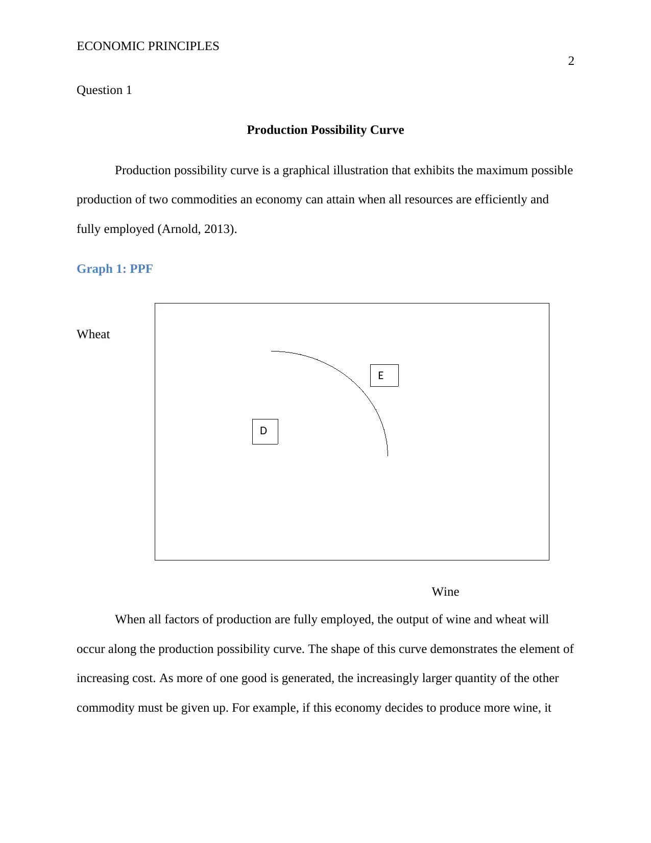
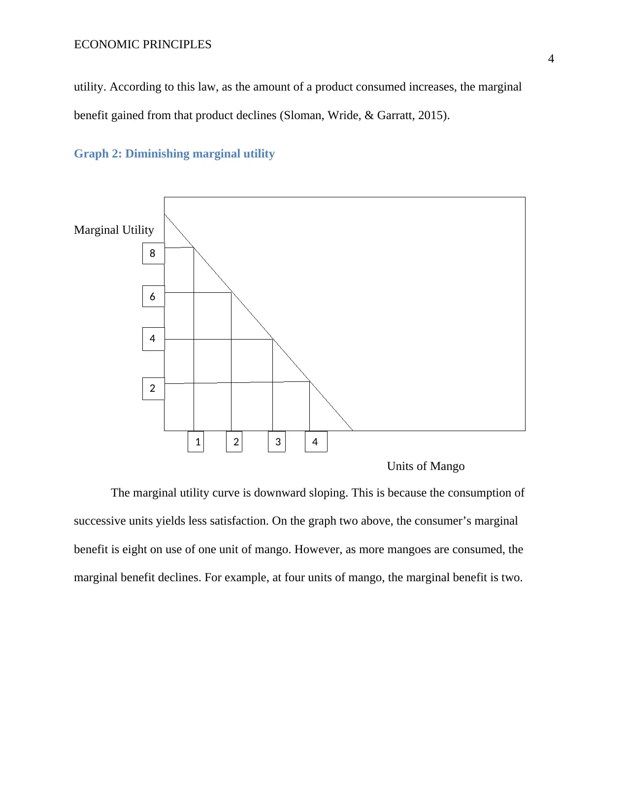
This economics assignment delves into core economic principles, providing a comprehensive analysis of production and market dynamics. The assignment begins by explaining the production possibility curve (PPC) and its implications, illustrating how it demonstrates the maximum possible production of two commodities with efficient resource allocation. It then explores the concept of opportunity cost, emphasizing how scarcity influences decision-making and resource allocation. The assignment further discusses marginal analysis, including marginal cost and marginal utility, and their roles in economic decision-making. The second part of the assignment focuses on demand and supply, defining 'quantity demanded' and 'demand schedule' and differentiating between 'movement along the demand curve' and 'shift in the demand curve'. Additionally, it analyzes market equilibrium, explaining excess demand and excess supply with the help of graphical illustrations. Overall, the assignment provides a solid foundation in fundamental economic concepts and their practical applications.

Running head: ECONOMIC PRINCIPLES
1
Economic Principles
Student’s name
Professor
Course
Date

ECONOMIC PRINCIPLES
2
Question 1
Production Possibility Curve
Production possibility curve is a graphical illustration that exhibits the maximum possible
production of two commodities an economy can attain when all resources are efficiently and
fully employed (Arnold, 2013).
Graph 1: PPF
Wheat
Wine
When all factors of production are fully employed, the output of wine and wheat will
occur along the production possibility curve. The shape of this curve demonstrates the element of
increasing cost. As more of one good is generated, the increasingly larger quantity of the other
commodity must be given up. For example, if this economy decides to produce more wine, it
D
E

ECONOMIC PRINCIPLES
3
will have to divert the resources of producing wheat to the production of wine. Therefore, less
wheat will be produced.
If an economy chooses to generate below capacity, say point D, then the combination of
wheat and wine would be less than what the country is capable of creating. However, the
combination of wheat and wine outside the curve, say point E, will not be possible because the
production level would surpass the capacity of the economy.
Opportunity Cost
The resources are often scarce and individuals must consider how to spend the limited
time or income. Opportunity cost arises when an economic agent decides between alternative
options of allocating limited resources. The opportunity cost of such choice is the price of the
next best different utilization of scarce resources (Sloman, Wride, & Garratt, 2015). On graph
one above, if there is no enhancement in productive resources, increasing the production of wine
has to entail reducing the generation of wheat because resources must be transferred from
production of wheat to wine. The sacrifice in the production of wheat is the opportunity cost.
Margin
In economics, the term margin refers to the value or utility of one extra unit of an item.
Marginal cost and marginal utility are some of essential concepts of margin. Marginal cost
entails a shift in total cost that results from generating an extra unit of output. Firms often make
use of marginal cost pricing where they equate the price to the marginal cost (Arnold, 2013). On
the other hand, marginal utility denotes the benefits gained from consuming or producing an
additional unit. Marginal benefit is commonly associated with the law of diminishing marginal

ECONOMIC PRINCIPLES
4
utility. According to this law, as the amount of a product consumed increases, the marginal
benefit gained from that product declines (Sloman, Wride, & Garratt, 2015).
Graph 2: Diminishing marginal utility
Marginal Utility
Units of Mango
The marginal utility curve is downward sloping. This is because the consumption of
successive units yields less satisfaction. On the graph two above, the consumer’s marginal
benefit is eight on use of one unit of mango. However, as more mangoes are consumed, the
marginal benefit declines. For example, at four units of mango, the marginal benefit is two.
1 2 3 4
8
6
4
2

ECONOMIC PRINCIPLES
5
Question 2
Quantity Demanded’ and ‘Demand Schedule’
Quantity demanded refers to total amount of a given good or a service that the buyers
purchase at any point in time. The quantity demanded is influenced by the price prevailing at the
marketplace. The extent at which quantity demanded shifts with respect to price is referred to as
elasticity of demand. On the other hand, demand schedule refers to a chart that displays the
number of products purchased at specific prices (Arnold, 2013). Also, demand schedule can be
described as a table that depicts the association between the price of commodities and a number
of goods clients are ready and able to buy.
‘Movement along demand curve’ and ‘shift in demand curve’
Graph 3: Movement along demand curve
Price
Quantity
Demand
P2
P1
Q1 Q2
A
B

ECONOMIC PRINCIPLES
6
Movement along demand curve refers to change in quantity demanded due to a change in
price. For example, move from point A to B is a downward movement resulting from a price
decline and shows an increase in demand.
On the other hand, a shift in demand curve is the change in demand due to a change in
non-price factors such as income and consumer preferences (Sloman, Wride, & Garratt, 2015).
The rightward shift shows an increase in demand and is caused by a favorable shift in non-price
factors. A leftward shift depicts a decline in demand results from an unfavorable change in non-
price factors.
Graph 4: Shift in demand curve
Price
Quantity
D1
P2
P1
Q1 Q2
D2

ECONOMIC PRINCIPLES
7
Graph 5: Commodity X
Price
Quantity
Market equilibrium occurs at point M where quantity demanded equals the quantity
supplied. If the price falls below Pe, say at P1, the quantity demanded is Q2 while the amount
supplied is Q1. Since the quantity demanded surpasses the quantity supplied, there will be excess
demand. On the other hand, if the price rises above Pe, say at P2, the amount demanded is Q1
while the amount supplied is Q2. Q2 exceeds Q1, and hence excess supply.
Pe
P2
P1
Qe Q2Q1
S
D
M
Excess Supply
Excess Demand

ECONOMIC PRINCIPLES
8
References
Arnold, R. A. (2013). Economics. Mason, Ohio: South-Western.
Sloman, J., Wride, A., & Garratt, D. (2015). Economics (9th ed.). Harlow : Pearson.