Economic Principles & Decision Making Report: ECON6000 Analysis
VerifiedAdded on 2023/05/28
|19
|4551
|122
Report
AI Summary
This report, prepared for ECON6000, analyzes the economic principles and decision-making processes involved in launching a new product, the Schmeckt Besser energy bar, in Atollia. The research department of Schmeckt Gut collected market data and information, which was then used to conduct a regression analysis. The report examines the impact of various economic variables, including income, inflation, unemployment, and tariffs, on the product's demand. It explores different scenarios and their effects on the market, providing recommendations and conclusions based on the analysis. The report also includes tables and figures illustrating the relationships between the variables and the demand for the product, offering a comprehensive overview of the economic factors influencing the product's success.
1
ECON6000 ECONOMIC PRINCIPLES & DECISION MAKING
ASSESSMENT 3- REPORT
ECON6000 ECONOMIC PRINCIPLES & DECISION MAKING
ASSESSMENT 3- REPORT
Paraphrase This Document
Need a fresh take? Get an instant paraphrase of this document with our AI Paraphraser
2
Executive summary
This paper contains a report directed to the board member of Schmeckt Gut which is looking
to launch a new product in the market. Under the process for the launch of the new product,
the research department of the company has collected market data and information. This
paper articulates projections of the chosen variable and finds out how the change of the
variable impacts the demand for the product.
3
Table of contents
1.0 Introduction..........................................................................................................................4
2.0 Methods................................................................................................................................4
3.0 Discussion............................................................................................................................4
4.0 Recommendations..............................................................................................................13
5.0 Conclusions........................................................................................................................14
Reference..................................................................................................................................15
⊘ This is a preview!⊘
Do you want full access?
Subscribe today to unlock all pages.
Trusted by 1+ million students worldwide
4
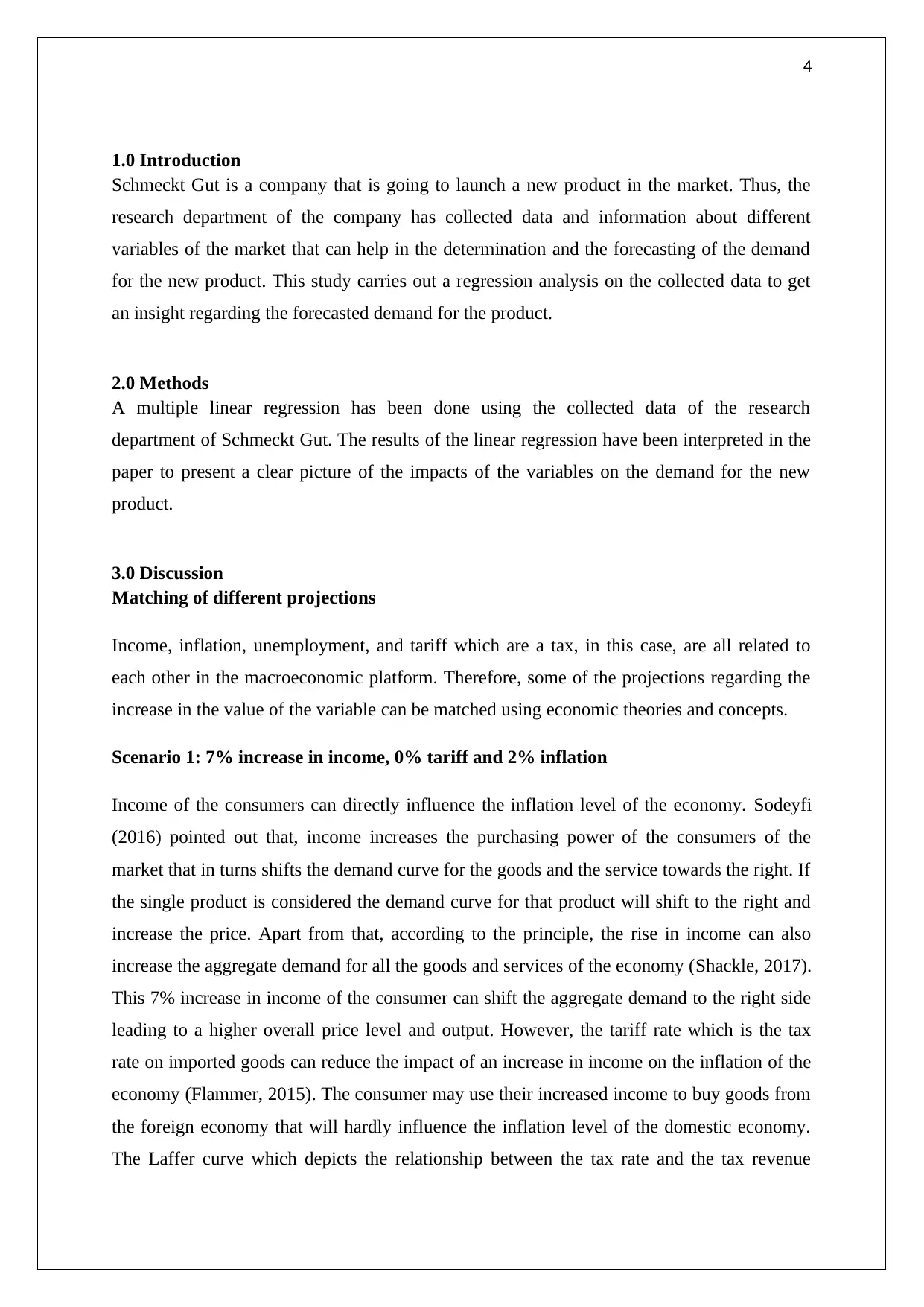
1.0 Introduction
Schmeckt Gut is a company that is going to launch a new product in the market. Thus, the
research department of the company has collected data and information about different
variables of the market that can help in the determination and the forecasting of the demand
for the new product. This study carries out a regression analysis on the collected data to get
an insight regarding the forecasted demand for the product.
2.0 Methods
A multiple linear regression has been done using the collected data of the research
department of Schmeckt Gut. The results of the linear regression have been interpreted in the
paper to present a clear picture of the impacts of the variables on the demand for the new
product.
3.0 Discussion
Matching of different projections
Income, inflation, unemployment, and tariff which are a tax, in this case, are all related to
each other in the macroeconomic platform. Therefore, some of the projections regarding the
increase in the value of the variable can be matched using economic theories and concepts.
Scenario 1: 7% increase in income, 0% tariff and 2% inflation
Income of the consumers can directly influence the inflation level of the economy. Sodeyfi
(2016) pointed out that, income increases the purchasing power of the consumers of the
market that in turns shifts the demand curve for the goods and the service towards the right. If
the single product is considered the demand curve for that product will shift to the right and
increase the price. Apart from that, according to the principle, the rise in income can also
increase the aggregate demand for all the goods and services of the economy (Shackle, 2017).
This 7% increase in income of the consumer can shift the aggregate demand to the right side
leading to a higher overall price level and output. However, the tariff rate which is the tax
rate on imported goods can reduce the impact of an increase in income on the inflation of the
economy (Flammer, 2015). The consumer may use their increased income to buy goods from
the foreign economy that will hardly influence the inflation level of the domestic economy.
The Laffer curve which depicts the relationship between the tax rate and the tax revenue
Paraphrase This Document
Need a fresh take? Get an instant paraphrase of this document with our AI Paraphraser
5
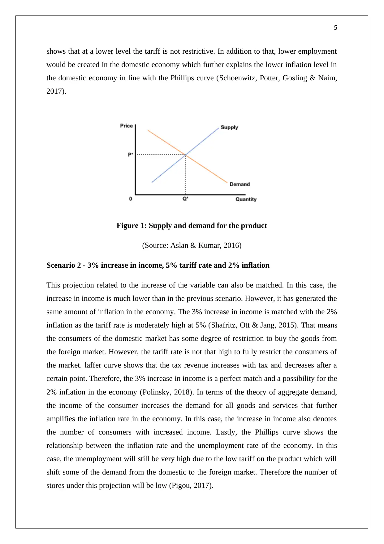
shows that at a lower level the tariff is not restrictive. In addition to that, lower employment
would be created in the domestic economy which further explains the lower inflation level in
the domestic economy in line with the Phillips curve (Schoenwitz, Potter, Gosling & Naim,
2017).
Figure 1: Supply and demand for the product
(Source: Aslan & Kumar, 2016)
Scenario 2 - 3% increase in income, 5% tariff rate and 2% inflation
This projection related to the increase of the variable can also be matched. In this case, the
increase in income is much lower than in the previous scenario. However, it has generated the
same amount of inflation in the economy. The 3% increase in income is matched with the 2%
inflation as the tariff rate is moderately high at 5% (Shafritz, Ott & Jang, 2015). That means
the consumers of the domestic market has some degree of restriction to buy the goods from
the foreign market. However, the tariff rate is not that high to fully restrict the consumers of
the market. laffer curve shows that the tax revenue increases with tax and decreases after a
certain point. Therefore, the 3% increase in income is a perfect match and a possibility for the
2% inflation in the economy (Polinsky, 2018). In terms of the theory of aggregate demand,
the income of the consumer increases the demand for all goods and services that further
amplifies the inflation rate in the economy. In this case, the increase in income also denotes
the number of consumers with increased income. Lastly, the Phillips curve shows the
relationship between the inflation rate and the unemployment rate of the economy. In this
case, the unemployment will still be very high due to the low tariff on the product which will
shift some of the demand from the domestic to the foreign market. Therefore the number of
stores under this projection will be low (Pigou, 2017).
6
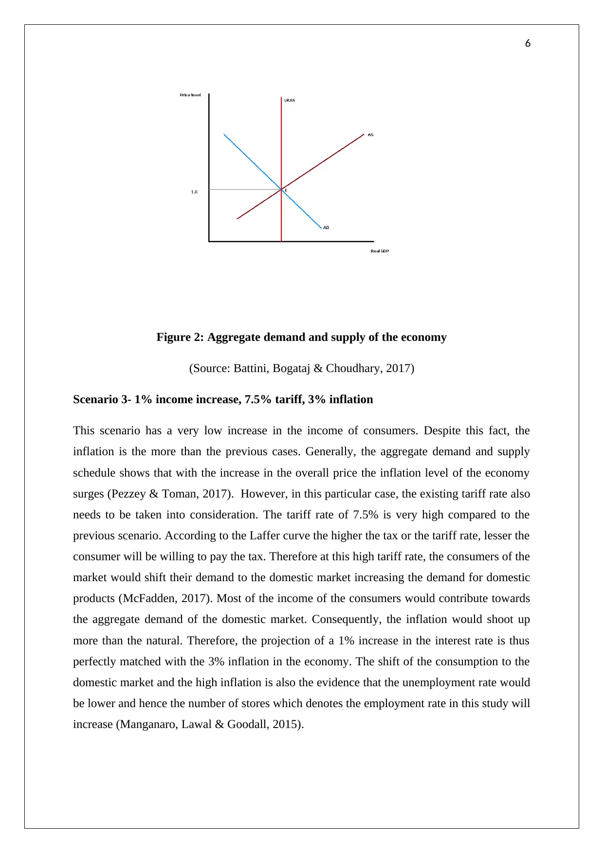
Figure 2: Aggregate demand and supply of the economy
(Source: Battini, Bogataj & Choudhary, 2017)
Scenario 3- 1% income increase, 7.5% tariff, 3% inflation
This scenario has a very low increase in the income of consumers. Despite this fact, the
inflation is the more than the previous cases. Generally, the aggregate demand and supply
schedule shows that with the increase in the overall price the inflation level of the economy
surges (Pezzey & Toman, 2017). However, in this particular case, the existing tariff rate also
needs to be taken into consideration. The tariff rate of 7.5% is very high compared to the
previous scenario. According to the Laffer curve the higher the tax or the tariff rate, lesser the
consumer will be willing to pay the tax. Therefore at this high tariff rate, the consumers of the
market would shift their demand to the domestic market increasing the demand for domestic
products (McFadden, 2017). Most of the income of the consumers would contribute towards
the aggregate demand of the domestic market. Consequently, the inflation would shoot up
more than the natural. Therefore, the projection of a 1% increase in the interest rate is thus
perfectly matched with the 3% inflation in the economy. The shift of the consumption to the
domestic market and the high inflation is also the evidence that the unemployment rate would
be lower and hence the number of stores which denotes the employment rate in this study will
increase (Manganaro, Lawal & Goodall, 2015).
⊘ This is a preview!⊘
Do you want full access?
Subscribe today to unlock all pages.
Trusted by 1+ million students worldwide
7
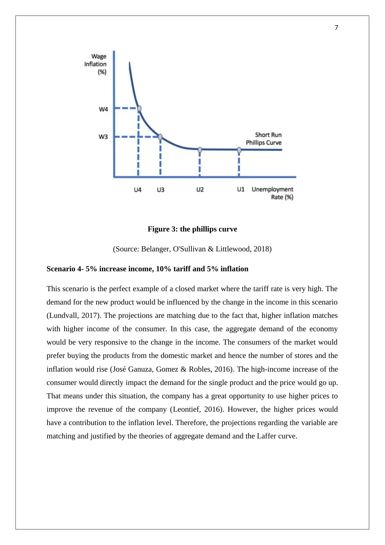
Figure 3: the phillips curve
(Source: Belanger, O'Sullivan & Littlewood, 2018)
Scenario 4- 5% increase income, 10% tariff and 5% inflation
This scenario is the perfect example of a closed market where the tariff rate is very high. The
demand for the new product would be influenced by the change in the income in this scenario
(Lundvall, 2017). The projections are matching due to the fact that, higher inflation matches
with higher income of the consumer. In this case, the aggregate demand of the economy
would be very responsive to the change in the income. The consumers of the market would
prefer buying the products from the domestic market and hence the number of stores and the
inflation would rise (José Ganuza, Gomez & Robles, 2016). The high-income increase of the
consumer would directly impact the demand for the single product and the price would go up.
That means under this situation, the company has a great opportunity to use higher prices to
improve the revenue of the company (Leontief, 2016). However, the higher prices would
have a contribution to the inflation level. Therefore, the projections regarding the variable are
matching and justified by the theories of aggregate demand and the Laffer curve.
Paraphrase This Document
Need a fresh take? Get an instant paraphrase of this document with our AI Paraphraser
8
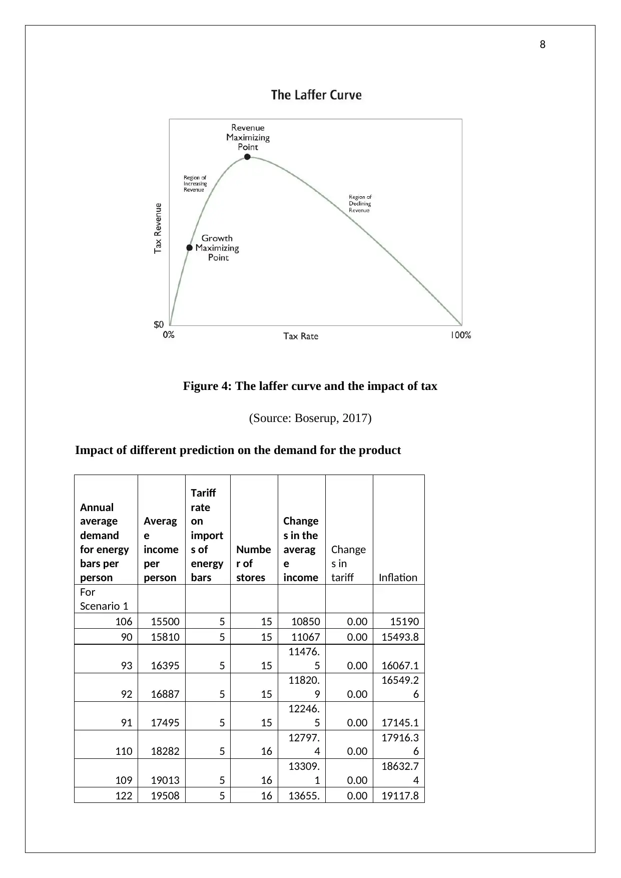
Figure 4: The laffer curve and the impact of tax
(Source: Boserup, 2017)
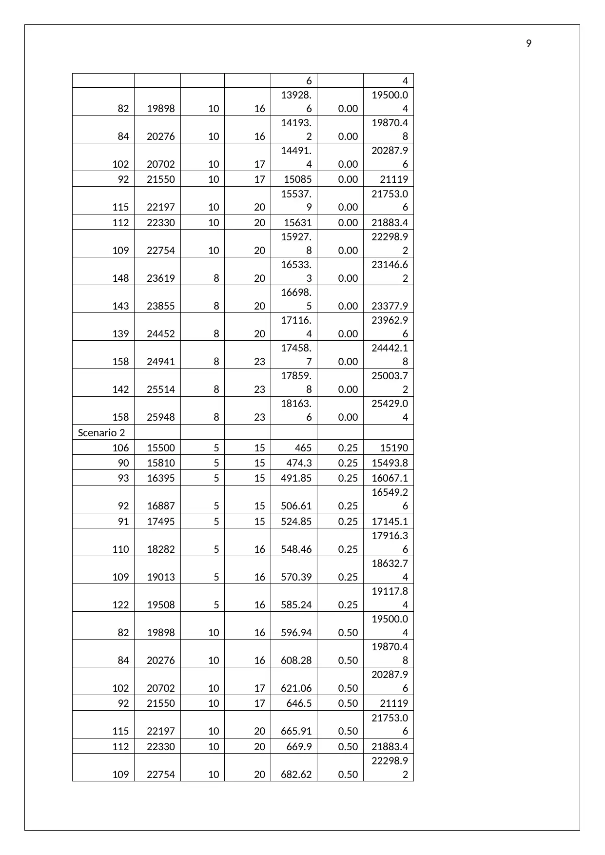
Impact of different prediction on the demand for the product
Annual
average
demand
for energy
bars per
person
Averag
e
income
per
person
Tariff
rate
on
import
s of
energy
bars
Numbe
r of
stores
Change
s in the
averag
e
income
Change
s in
tariff Inflation
For
Scenario 1
106 15500 5 15 10850 0.00 15190
90 15810 5 15 11067 0.00 15493.8
93 16395 5 15
11476.
5 0.00 16067.1
92 16887 5 15
11820.
9 0.00
16549.2
6
91 17495 5 15
12246.
5 0.00 17145.1
110 18282 5 16
12797.
4 0.00
17916.3
6
109 19013 5 16
13309.
1 0.00
18632.7
4
122 19508 5 16 13655. 0.00 19117.8
Figure 4: The laffer curve and the impact of tax
(Source: Boserup, 2017)
Impact of different prediction on the demand for the product
Annual
average
demand
for energy
bars per
person
Averag
e
income
per
person
Tariff
rate
on
import
s of
energy
bars
Numbe
r of
stores
Change
s in the
averag
e
income
Change
s in
tariff Inflation
For
Scenario 1
106 15500 5 15 10850 0.00 15190
90 15810 5 15 11067 0.00 15493.8
93 16395 5 15
11476.
5 0.00 16067.1
92 16887 5 15
11820.
9 0.00
16549.2
6
91 17495 5 15
12246.
5 0.00 17145.1
110 18282 5 16
12797.
4 0.00
17916.3
6
109 19013 5 16
13309.
1 0.00
18632.7
4
122 19508 5 16 13655. 0.00 19117.8
9
6 4
82 19898 10 16
13928.
6 0.00
19500.0
4
84 20276 10 16
14193.
2 0.00
19870.4
8
102 20702 10 17
14491.
4 0.00
20287.9
6
92 21550 10 17 15085 0.00 21119
115 22197 10 20
15537.
9 0.00
21753.0
6
112 22330 10 20 15631 0.00 21883.4
109 22754 10 20
15927.
8 0.00
22298.9
2
148 23619 8 20
16533.
3 0.00
23146.6
2
143 23855 8 20
16698.
5 0.00 23377.9
139 24452 8 20
17116.
4 0.00
23962.9
6
158 24941 8 23
17458.
7 0.00
24442.1
8
142 25514 8 23
17859.
8 0.00
25003.7
2
158 25948 8 23
18163.
6 0.00
25429.0
4
Scenario 2
106 15500 5 15 465 0.25 15190
90 15810 5 15 474.3 0.25 15493.8
93 16395 5 15 491.85 0.25 16067.1
92 16887 5 15 506.61 0.25
16549.2
6
91 17495 5 15 524.85 0.25 17145.1
110 18282 5 16 548.46 0.25
17916.3
6
109 19013 5 16 570.39 0.25
18632.7
4
122 19508 5 16 585.24 0.25
19117.8
4
82 19898 10 16 596.94 0.50
19500.0
4
84 20276 10 16 608.28 0.50
19870.4
8
102 20702 10 17 621.06 0.50
20287.9
6
92 21550 10 17 646.5 0.50 21119
115 22197 10 20 665.91 0.50
21753.0
6
112 22330 10 20 669.9 0.50 21883.4
109 22754 10 20 682.62 0.50
22298.9
2
⊘ This is a preview!⊘
Do you want full access?
Subscribe today to unlock all pages.
Trusted by 1+ million students worldwide
10
148 23619 8 20 708.57 0.38
23146.6
2
143 23855 8 20 715.65 0.38 23377.9
139 24452 8 20 733.56 0.38
23962.9
6
158 24941 8 23 748.23 0.38
24442.1
8
142 25514 8 23 765.42 0.38
25003.7
2
158 25948 8 23 778.44 0.38
25429.0
4
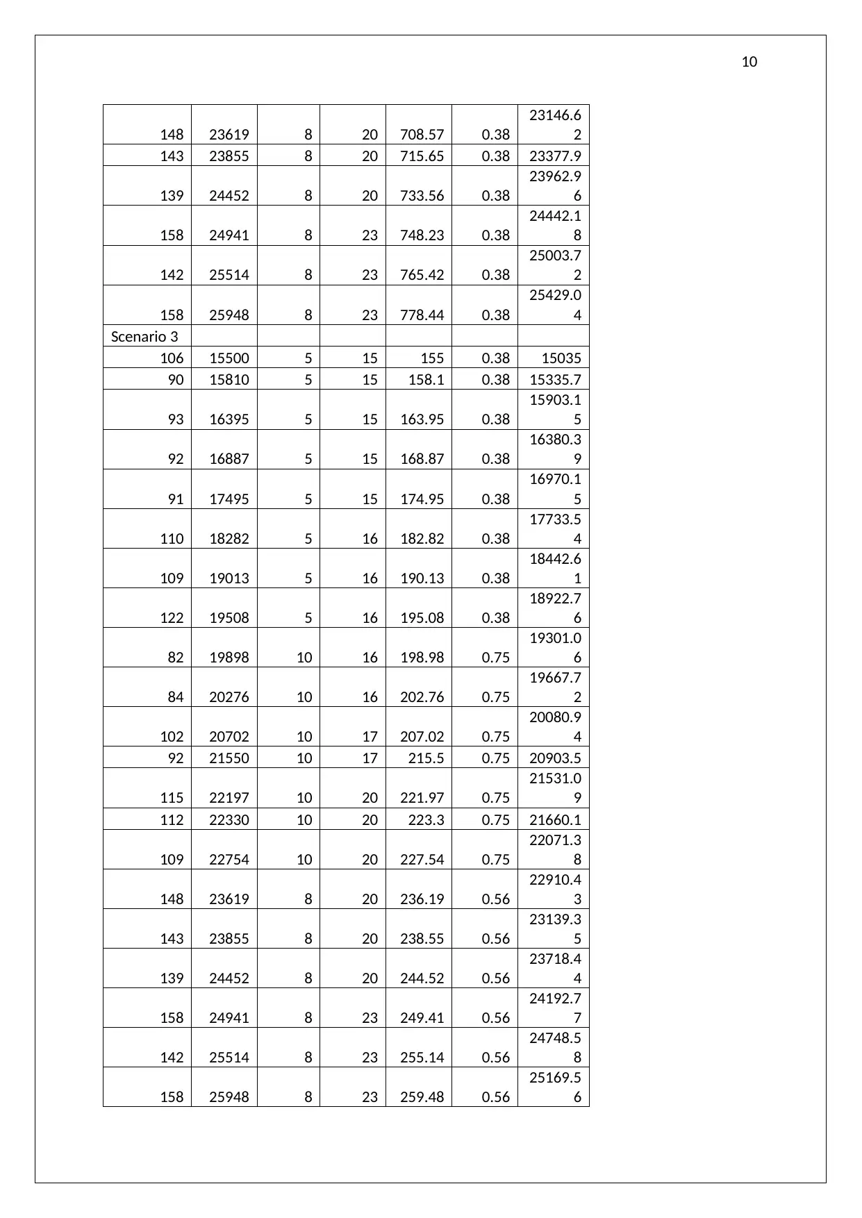
Scenario 3
106 15500 5 15 155 0.38 15035
90 15810 5 15 158.1 0.38 15335.7
93 16395 5 15 163.95 0.38
15903.1
5
92 16887 5 15 168.87 0.38
16380.3
9
91 17495 5 15 174.95 0.38
16970.1
5
110 18282 5 16 182.82 0.38
17733.5
4
109 19013 5 16 190.13 0.38
18442.6
1
122 19508 5 16 195.08 0.38
18922.7
6
82 19898 10 16 198.98 0.75
19301.0
6
84 20276 10 16 202.76 0.75
19667.7
2
102 20702 10 17 207.02 0.75
20080.9
4
92 21550 10 17 215.5 0.75 20903.5
115 22197 10 20 221.97 0.75
21531.0
9
112 22330 10 20 223.3 0.75 21660.1
109 22754 10 20 227.54 0.75
22071.3
8
148 23619 8 20 236.19 0.56
22910.4
3
143 23855 8 20 238.55 0.56
23139.3
5
139 24452 8 20 244.52 0.56
23718.4
4
158 24941 8 23 249.41 0.56
24192.7
7
142 25514 8 23 255.14 0.56
24748.5
8
158 25948 8 23 259.48 0.56
25169.5
6
148 23619 8 20 708.57 0.38
23146.6
2
143 23855 8 20 715.65 0.38 23377.9
139 24452 8 20 733.56 0.38
23962.9
6
158 24941 8 23 748.23 0.38
24442.1
8
142 25514 8 23 765.42 0.38
25003.7
2
158 25948 8 23 778.44 0.38
25429.0
4
Scenario 3
106 15500 5 15 155 0.38 15035
90 15810 5 15 158.1 0.38 15335.7
93 16395 5 15 163.95 0.38
15903.1
5
92 16887 5 15 168.87 0.38
16380.3
9
91 17495 5 15 174.95 0.38
16970.1
5
110 18282 5 16 182.82 0.38
17733.5
4
109 19013 5 16 190.13 0.38
18442.6
1
122 19508 5 16 195.08 0.38
18922.7
6
82 19898 10 16 198.98 0.75
19301.0
6
84 20276 10 16 202.76 0.75
19667.7
2
102 20702 10 17 207.02 0.75
20080.9
4
92 21550 10 17 215.5 0.75 20903.5
115 22197 10 20 221.97 0.75
21531.0
9
112 22330 10 20 223.3 0.75 21660.1
109 22754 10 20 227.54 0.75
22071.3
8
148 23619 8 20 236.19 0.56
22910.4
3
143 23855 8 20 238.55 0.56
23139.3
5
139 24452 8 20 244.52 0.56
23718.4
4
158 24941 8 23 249.41 0.56
24192.7
7
142 25514 8 23 255.14 0.56
24748.5
8
158 25948 8 23 259.48 0.56
25169.5
6
Paraphrase This Document
Need a fresh take? Get an instant paraphrase of this document with our AI Paraphraser
11
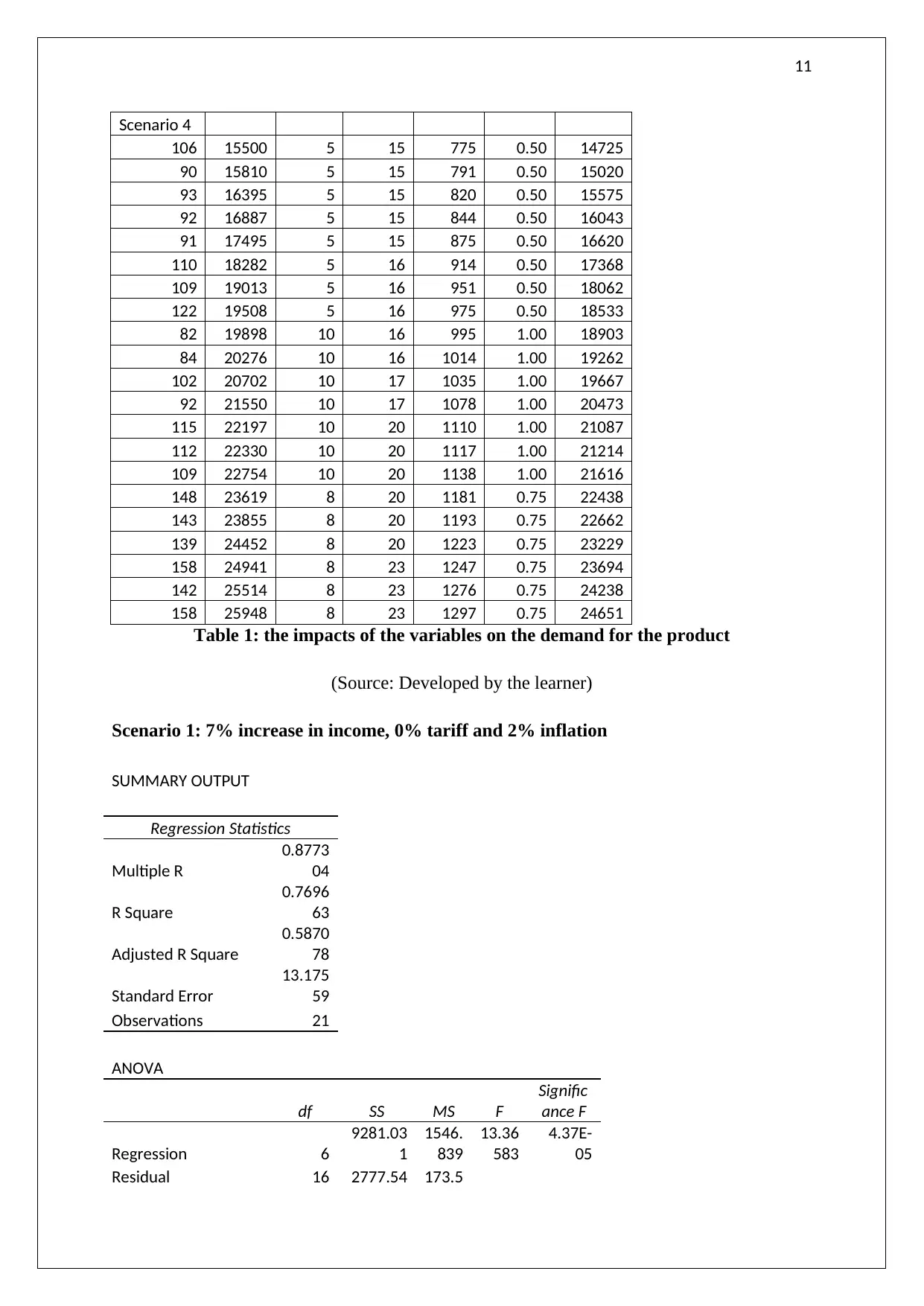
Scenario 4
106 15500 5 15 775 0.50 14725
90 15810 5 15 791 0.50 15020
93 16395 5 15 820 0.50 15575
92 16887 5 15 844 0.50 16043
91 17495 5 15 875 0.50 16620
110 18282 5 16 914 0.50 17368
109 19013 5 16 951 0.50 18062
122 19508 5 16 975 0.50 18533
82 19898 10 16 995 1.00 18903
84 20276 10 16 1014 1.00 19262
102 20702 10 17 1035 1.00 19667
92 21550 10 17 1078 1.00 20473
115 22197 10 20 1110 1.00 21087
112 22330 10 20 1117 1.00 21214
109 22754 10 20 1138 1.00 21616
148 23619 8 20 1181 0.75 22438
143 23855 8 20 1193 0.75 22662
139 24452 8 20 1223 0.75 23229
158 24941 8 23 1247 0.75 23694
142 25514 8 23 1276 0.75 24238
158 25948 8 23 1297 0.75 24651
Table 1: the impacts of the variables on the demand for the product
(Source: Developed by the learner)
Scenario 1: 7% increase in income, 0% tariff and 2% inflation
SUMMARY OUTPUT
Regression Statistics
Multiple R
0.8773
04
R Square
0.7696
63
Adjusted R Square
0.5870
78
Standard Error
13.175
59
Observations 21
ANOVA
df SS MS F
Signific
ance F
Regression 6
9281.03
1
1546.
839
13.36
583
4.37E-
05
Residual 16 2777.54 173.5
12
963
Total 22
12058.5
7
Coeffic
ients
Standar
d Error t Stat
P-
value
Lower
95%
Upper
95%
Lower
95.0%
Upper
95.0%
Intercept 5824
4.04E+0
8
1.44E
-05
0.999
989
-
8.6E+08
8.56E
+08
-
8.6E+0
8
8.56E+
08
Average income per
person
-
1.9E+1
2
2.65E+1
2
-
0.728
94
0.476
573
-
7.6E+12
3.69E
+12
-
7.6E+1
2
3.69E+
12
Tariff rate on imports
of energy bars
-
655.36
7
367.450
9
-
1.783
55
0.093
474
-
1434.33
123.5
939
-
1434.3
3
123.59
39
Number of stores
2.2321
78
4.39073
5
0.508
384
0.618
122
-
7.07576
11.54
012
-
7.0757
6
11.540
12
Changes in the
average income 0 0
6553
5
#NU
M! 0 0 0 0
Changes in tariff 0 0
6553
5
#NU
M! 0 0 0 0
Inflation
1.97E+
12
2.71E+1
2
0.728
942
0.476
573
-
3.8E+12
7.71E
+12
-
3.8E+1
2
7.71E+
12
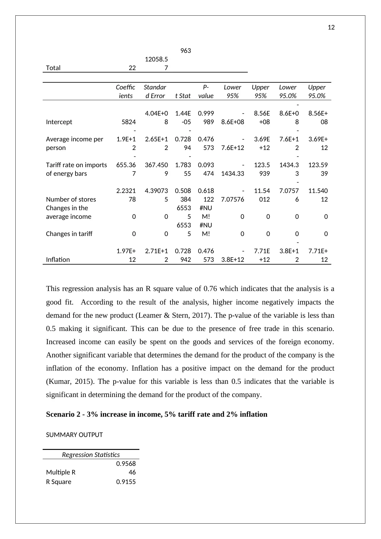
This regression analysis has an R square value of 0.76 which indicates that the analysis is a
good fit. According to the result of the analysis, higher income negatively impacts the
demand for the new product (Leamer & Stern, 2017). The p-value of the variable is less than
0.5 making it significant. This can be due to the presence of free trade in this scenario.
Increased income can easily be spent on the goods and services of the foreign economy.
Another significant variable that determines the demand for the product of the company is the
inflation of the economy. Inflation has a positive impact on the demand for the product
(Kumar, 2015). The p-value for this variable is less than 0.5 indicates that the variable is
significant in determining the demand for the product of the company.
Scenario 2 - 3% increase in income, 5% tariff rate and 2% inflation
SUMMARY OUTPUT
Regression Statistics
Multiple R
0.9568
46
R Square 0.9155
963
Total 22
12058.5
7
Coeffic
ients
Standar
d Error t Stat
P-
value
Lower
95%
Upper
95%
Lower
95.0%
Upper
95.0%
Intercept 5824
4.04E+0
8
1.44E
-05
0.999
989
-
8.6E+08
8.56E
+08
-
8.6E+0
8
8.56E+
08
Average income per
person
-
1.9E+1
2
2.65E+1
2
-
0.728
94
0.476
573
-
7.6E+12
3.69E
+12
-
7.6E+1
2
3.69E+
12
Tariff rate on imports
of energy bars
-
655.36
7
367.450
9
-
1.783
55
0.093
474
-
1434.33
123.5
939
-
1434.3
3
123.59
39
Number of stores
2.2321
78
4.39073
5
0.508
384
0.618
122
-
7.07576
11.54
012
-
7.0757
6
11.540
12
Changes in the
average income 0 0
6553
5
#NU
M! 0 0 0 0
Changes in tariff 0 0
6553
5
#NU
M! 0 0 0 0
Inflation
1.97E+
12
2.71E+1
2
0.728
942
0.476
573
-
3.8E+12
7.71E
+12
-
3.8E+1
2
7.71E+
12
This regression analysis has an R square value of 0.76 which indicates that the analysis is a
good fit. According to the result of the analysis, higher income negatively impacts the
demand for the new product (Leamer & Stern, 2017). The p-value of the variable is less than
0.5 making it significant. This can be due to the presence of free trade in this scenario.
Increased income can easily be spent on the goods and services of the foreign economy.
Another significant variable that determines the demand for the product of the company is the
inflation of the economy. Inflation has a positive impact on the demand for the product
(Kumar, 2015). The p-value for this variable is less than 0.5 indicates that the variable is
significant in determining the demand for the product of the company.
Scenario 2 - 3% increase in income, 5% tariff rate and 2% inflation
SUMMARY OUTPUT
Regression Statistics
Multiple R
0.9568
46
R Square 0.9155
⊘ This is a preview!⊘
Do you want full access?
Subscribe today to unlock all pages.
Trusted by 1+ million students worldwide
1 out of 19
Related Documents


Your All-in-One AI-Powered Toolkit for Academic Success.
+13062052269
info@desklib.com
Available 24*7 on WhatsApp / Email
![[object Object]](/_next/static/media/star-bottom.7253800d.svg)
Unlock your academic potential
Copyright © 2020–2026 A2Z Services. All Rights Reserved. Developed and managed by ZUCOL.