Economics Assignment Solution: Chapters 2, 3, and 9 Analysis

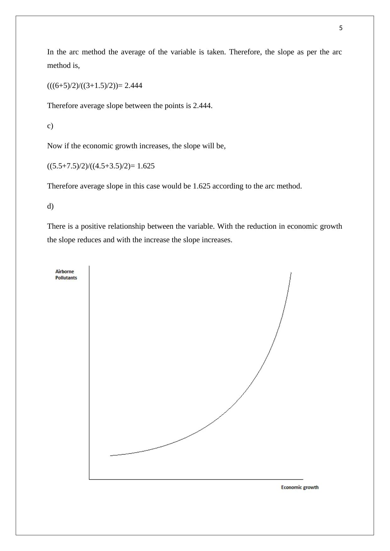
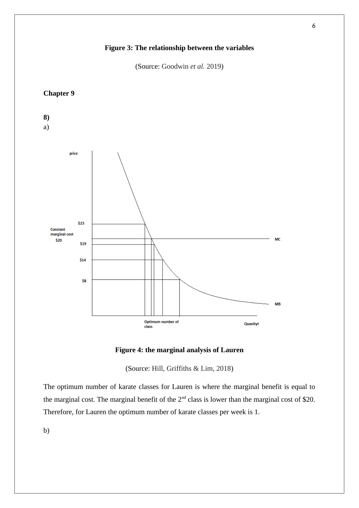
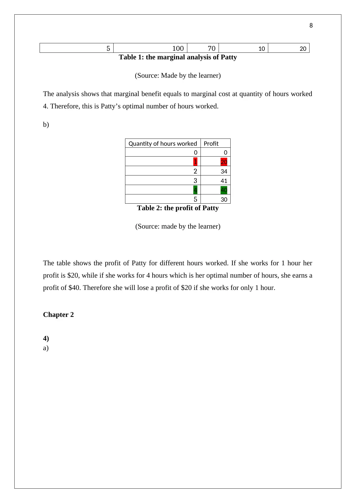
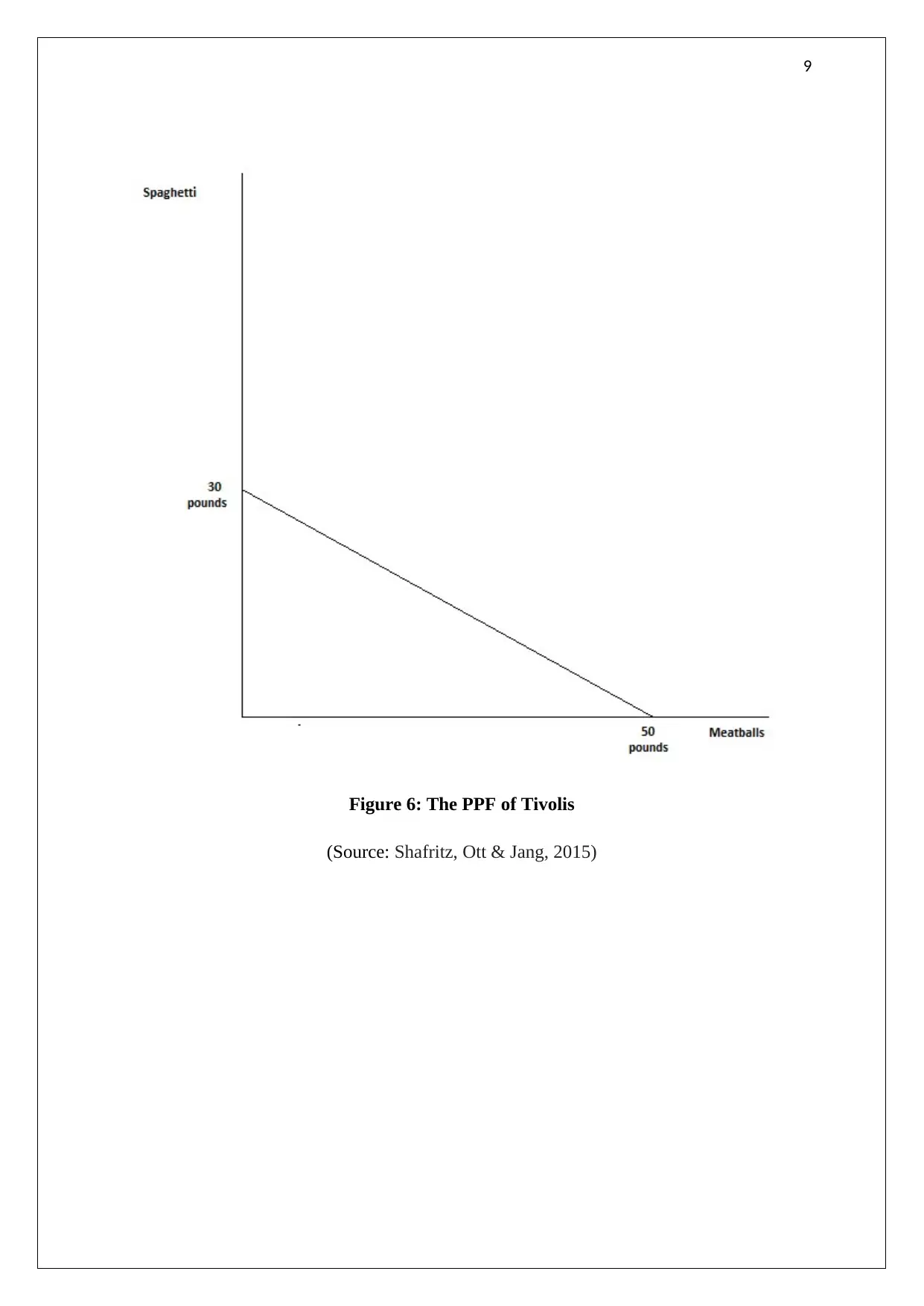
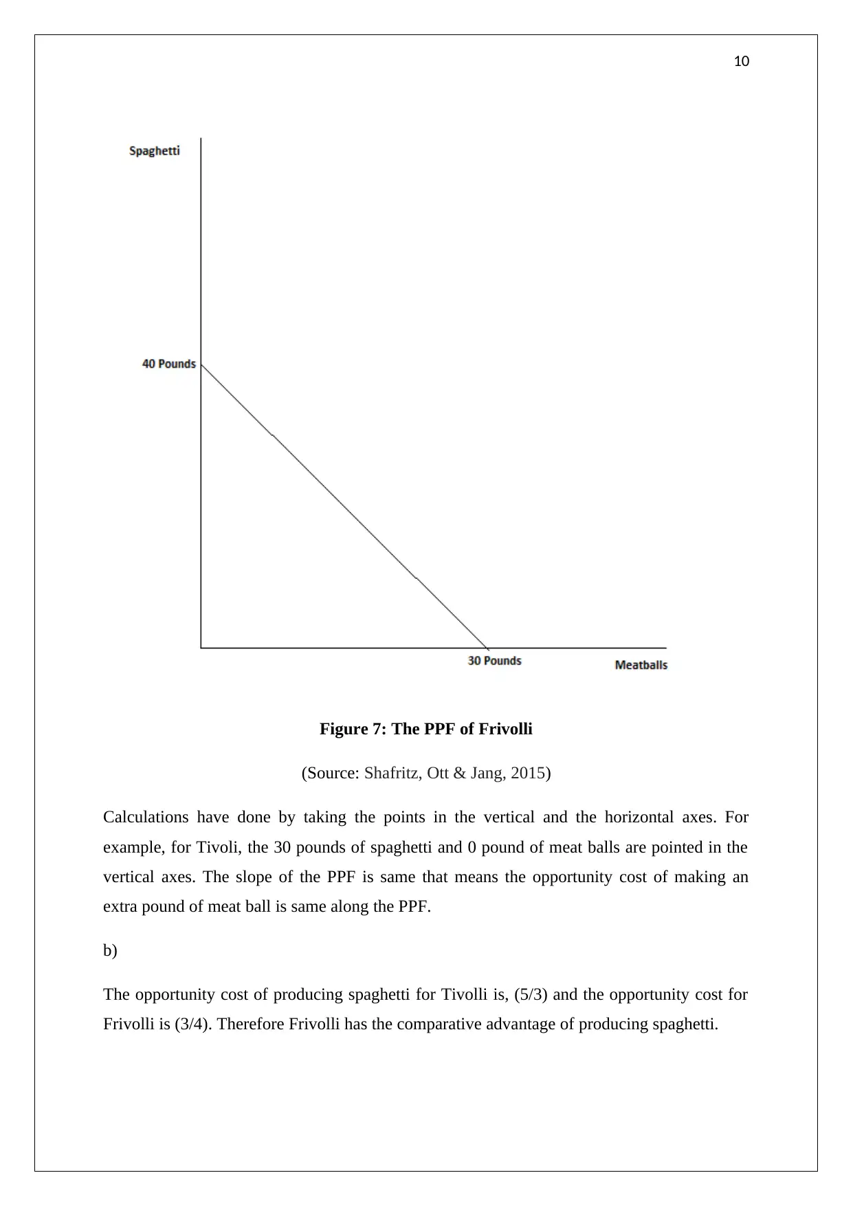
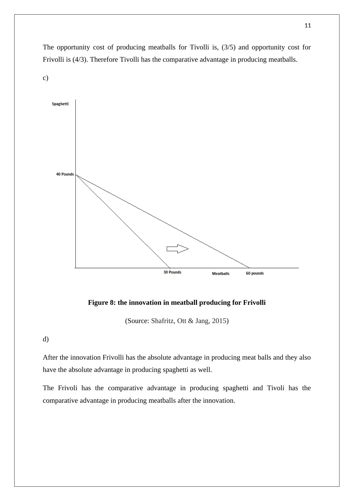
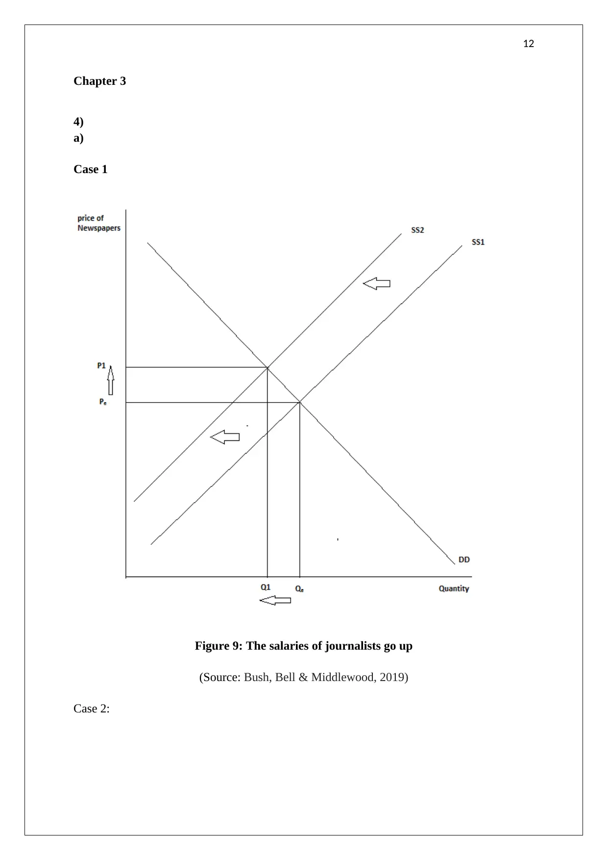
This economics assignment solution covers key concepts from Chapters 2, 3, and 9. It includes schematic diagrams illustrating relationships between variables, such as economic growth and airborne pollutants, and analyzes curves with changing slopes. The assignment delves into marginal analysis, determining optimal karate class numbers for individuals, and examines the relationship between hours worked and profit. Furthermore, the solution explores production possibility frontiers (PPF) and comparative advantage, along with the impact of innovation. It also addresses supply and demand scenarios, illustrating how changes in salaries, news events, and other factors affect market equilibrium. The assignment utilizes diagrams and calculations to explain the economic concepts.

1
ECONOMICS ASSIGNMENT

2
Contents
Chapter 2 Appendix...................................................................................................................3
4)................................................................................................................................................3
8)................................................................................................................................................4
Chapter 9....................................................................................................................................6
8)................................................................................................................................................6
10)..............................................................................................................................................7
Chapter 2....................................................................................................................................8
4)................................................................................................................................................8
Chapter 3..................................................................................................................................12
4)..............................................................................................................................................12
16)............................................................................................................................................17
Reference..................................................................................................................................21

3
Chapter 2 Appendix
4)
a)
Figure 1: The schematic diagram
(Source: Developed by the learner)
This is a concave curve that shows the relationship between the two variables. The variables
are negatively related to each other where the changes in Y increases more with the further
changes in X as shown in the figure. That means the slope of the curve is increasing along the
horizontal axis.
(b)

4
Figure 2: The Schematic diagram
(Source: Developed by the learner)
The slope is reducing along the horizontal axis and hence the curve is an inverted U-shaped
curve. Therefore, the curve has a maximum point.
8)
a) In this case, the independent variable is the economic growth. The dependant variable in
this case is the airborne pollutants. The independent variable explains the changes in the
dependant variable.
b)

5
In the arc method the average of the variable is taken. Therefore, the slope as per the arc
method is,
(((6+5)/2)/((3+1.5)/2))= 2.444
Therefore average slope between the points is 2.444.
c)
Now if the economic growth increases, the slope will be,
((5.5+7.5)/2)/((4.5+3.5)/2)= 1.625
Therefore average slope in this case would be 1.625 according to the arc method.
d)
There is a positive relationship between the variable. With the reduction in economic growth
the slope reduces and with the increase the slope increases.

6
Figure 3: The relationship between the variables
(Source: Goodwin et al. 2019)
Chapter 9
8)
a)
Figure 4: the marginal analysis of Lauren
(Source: Hill, Griffiths & Lim, 2018)
The optimum number of karate classes for Lauren is where the marginal benefit is equal to
the marginal cost. The marginal benefit of the 2nd class is lower than the marginal cost of $20.
Therefore, for Lauren the optimum number of karate classes per week is 1.
b)

7
Figure 5: the marginal analysis of Georgia
(Source: Hill, Griffiths & Lim, 2018)
In the case of Georgia, the marginal cost is same, $20. The marginal benefit of the 2nd class is
$22 which is higher than the marginal cost. However, the marginal benefit of the 3rd class is
lower than the marginal cost and hence the optimal number of classes of karate par week for
Georgia is 2.
10)
a)
Quantity of hours
worked Total benefit
Total
cost
marginal
benefit
marginal
cost
0 0 0
1 30 10 30 10
2 55 21 25 11
3 75 34 20 13
4 90 50 15 16

8
5 100 70 10 20
Table 1: the marginal analysis of Patty
(Source: Made by the learner)
The analysis shows that marginal benefit equals to marginal cost at quantity of hours worked
4. Therefore, this is Patty’s optimal number of hours worked.
b)
Quantity of hours worked Profit
0 0
1 20
2 34
3 41
4 40
5 30
Table 2: the profit of Patty
(Source: made by the learner)
The table shows the profit of Patty for different hours worked. If she works for 1 hour her
profit is $20, while if she works for 4 hours which is her optimal number of hours, she earns a
profit of $40. Therefore she will lose a profit of $20 if she works for only 1 hour.
Chapter 2
4)
a)

9
Figure 6: The PPF of Tivolis
(Source: Shafritz, Ott & Jang, 2015)

10
Figure 7: The PPF of Frivolli
(Source: Shafritz, Ott & Jang, 2015)
Calculations have done by taking the points in the vertical and the horizontal axes. For
example, for Tivoli, the 30 pounds of spaghetti and 0 pound of meat balls are pointed in the
vertical axes. The slope of the PPF is same that means the opportunity cost of making an
extra pound of meat ball is same along the PPF.
b)
The opportunity cost of producing spaghetti for Tivolli is, (5/3) and the opportunity cost for
Frivolli is (3/4). Therefore Frivolli has the comparative advantage of producing spaghetti.

11
The opportunity cost of producing meatballs for Tivolli is, (3/5) and opportunity cost for
Frivolli is (4/3). Therefore Tivolli has the comparative advantage in producing meatballs.
c)
Figure 8: the innovation in meatball producing for Frivolli
(Source: Shafritz, Ott & Jang, 2015)
d)
After the innovation Frivolli has the absolute advantage in producing meat balls and they also
have the absolute advantage in producing spaghetti as well.
The Frivoli has the comparative advantage in producing spaghetti and Tivoli has the
comparative advantage in producing meatballs after the innovation.

12
Chapter 3
4)
a)
Case 1
Figure 9: The salaries of journalists go up
(Source: Bush, Bell & Middlewood, 2019)
Case 2:

13
Figure 10: There is a big news event in your town, which is reported in the newspapers.
(Source: Bush, Bell & Middlewood, 2019)
b)
Case 1

14
Figure 11: The Rams win the super bowl
(Source: Bush, Bell & Middlewood, 2019)
Case 2

15
Figure 12: The price of cotton increases
(Source: Goodwin et al. 2019)
c)
Case 1

16
Figure 13: People realize how fattening bagels are
(Source: Goodwin et al. 2019)
Case 2

17
Figure 14: People have less time to make themselves a cooked
(Source: Goodwin et al. 2019)
16)
a)

18
Figure 15: The increase in demand in babysitting market
(Source: Bush, Bell & Middlewood, 2019)
b)

19
Figure 16: The babysitting market after 14 years
(Source: Bush, Bell & Middlewood, 2019)
c)

20
Figure 17: The babysitting market after 30 years
(Source: Bush, Bell & Middlewood, 2019)

21
Reference
Bush, T., Bell, L., & Middlewood, D. (Eds.). (2019). Principles of Educational Leadership &
Management. SAGE Publications Limited.
Goodwin, N., Harris, J. M., Nelson, J. A., Roach, B., & Torras, M. (2019). Principles of
economics in context. Routledge.
Hill, R. C., Griffiths, W. E., & Lim, G. C. (2018). Principles of econometrics. John Wiley &
Sons.
Shafritz, J. M., Ott, J. S., & Jang, Y. S. (2015). Classics of organization theory. Cengage
Learning.