Economics for Business: Assignment Solution - Concepts and Analysis
VerifiedAdded on 2022/12/28
|23
|5441
|9
Homework Assignment
AI Summary
This economics assignment solution covers key concepts in both microeconomics and macroeconomics. The solution begins with an analysis of demand and supply, including the calculation of price elasticity of demand using the midpoint formula for petrol and air conditioners, and discusses the incidence of tax under elastic and inelastic demand conditions. It then moves on to production costs, differentiating between accounting and economic profit and provides advice for a business owner. The assignment also explores market structures, specifically focusing on a monopoly firm, discussing its demand curve characteristics, the benefits for a company, and the implications for consumers in both the short and long run. Finally, it addresses macroeconomic topics such as GDP, aggregate demand, and money supply within an economy. The assessment includes calculations, explanations, and analyses of various economic principles.
Economics for Business
1
1
Paraphrase This Document
Need a fresh take? Get an instant paraphrase of this document with our AI Paraphraser
Table of Contents
Introduction......................................................................................................................................3
Assessment Question Week 2 and 3 – Demand and Supply, and Elasticity....................................3
Question1....................................................................................................................................3
Assessment Question Week 4 – Production Costs..........................................................................7
Question 2...................................................................................................................................7
Assessment Question Week 5 and 6 – Market Structure.................................................................8
Question 3...................................................................................................................................8
Assessment Question Week 7 and 8 – Measuring the size of the economy..................................11
Question 4.................................................................................................................................11
Assessment Question Week 9 and 10: Inflation and unemployment, and Macro economics.......14
Question 5.................................................................................................................................14
Assessment Question Week 11......................................................................................................17
Question 6.................................................................................................................................17
Conclusion.....................................................................................................................................19
References......................................................................................................................................21
2
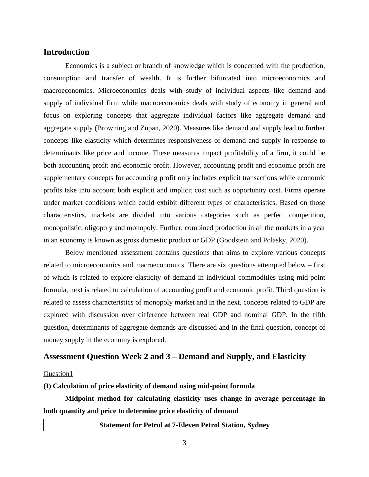
Introduction
Economics is a subject or branch of knowledge which is concerned with the production,
consumption and transfer of wealth. It is further bifurcated into microeconomics and
macroeconomics. Microeconomics deals with study of individual aspects like demand and
supply of individual firm while macroeconomics deals with study of economy in general and
focus on exploring concepts that aggregate individual factors like aggregate demand and
aggregate supply (Browning and Zupan, 2020). Measures like demand and supply lead to further
concepts like elasticity which determines responsiveness of demand and supply in response to
determinants like price and income. These measures impact profitability of a firm, it could be
both accounting profit and economic profit. However, accounting profit and economic profit are
supplementary concepts for accounting profit only includes explicit transactions while economic
profits take into account both explicit and implicit cost such as opportunity cost. Firms operate
under market conditions which could exhibit different types of characteristics. Based on those
characteristics, markets are divided into various categories such as perfect competition,
monopolistic, oligopoly and monopoly. Further, combined production in all the markets in a year
in an economy is known as gross domestic product or GDP (Goodstein and Polasky, 2020).
Below mentioned assessment contains questions that aims to explore various concepts
related to microeconomics and macroeconomics. There are six questions attempted below – first
of which is related to explore elasticity of demand in individual commodities using mid-point
formula, next is related to calculation of accounting profit and economic profit. Third question is
related to assess characteristics of monopoly market and in the next, concepts related to GDP are
explored with discussion over difference between real GDP and nominal GDP. In the fifth
question, determinants of aggregate demands are discussed and in the final question, concept of
money supply in the economy is explored.
Assessment Question Week 2 and 3 – Demand and Supply, and Elasticity
Question1
(I) Calculation of price elasticity of demand using mid-point formula
Midpoint method for calculating elasticity uses change in average percentage in
both quantity and price to determine price elasticity of demand
Statement for Petrol at 7-Eleven Petrol Station, Sydney
3
⊘ This is a preview!⊘
Do you want full access?
Subscribe today to unlock all pages.
Trusted by 1+ million students worldwide
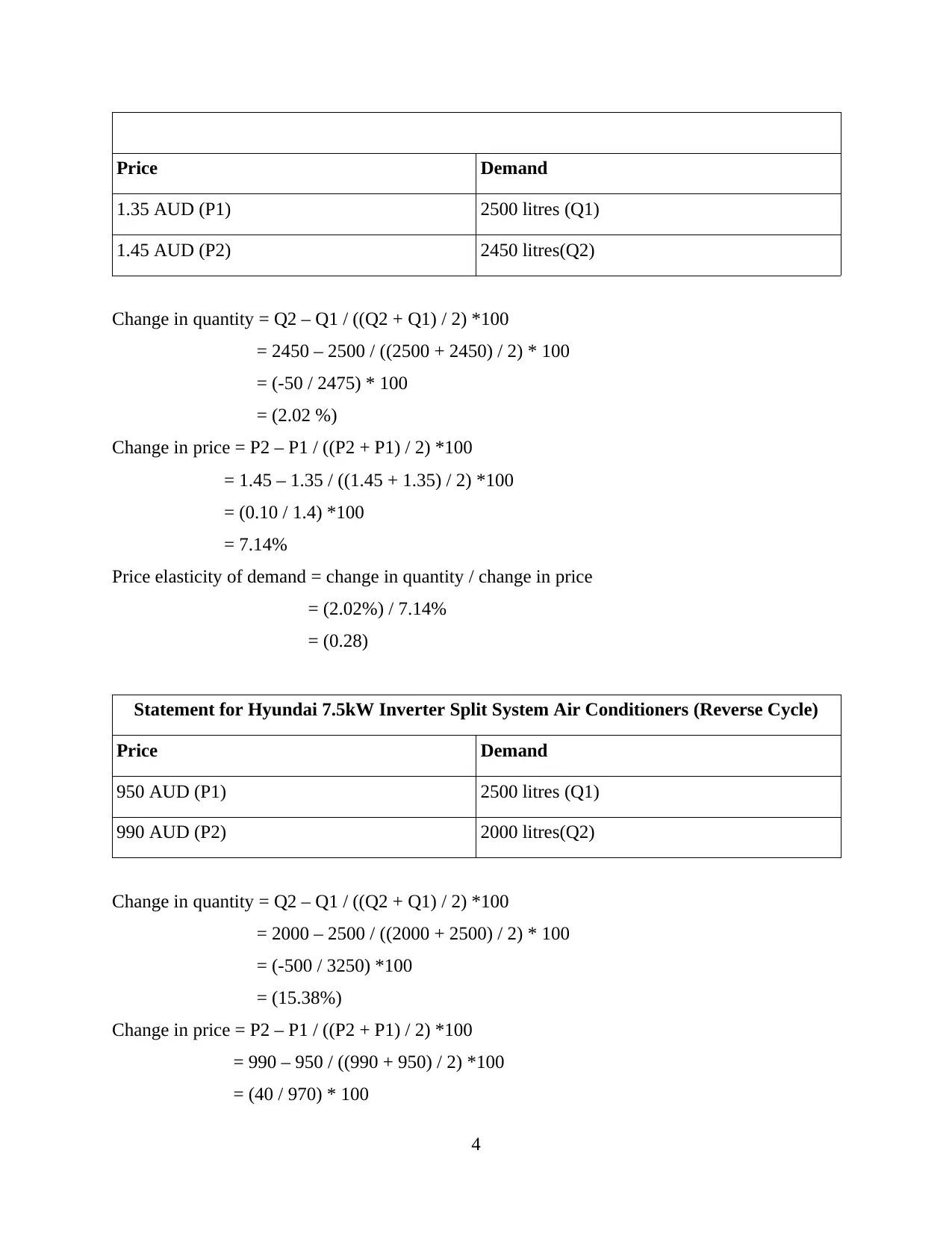
Price Demand
1.35 AUD (P1) 2500 litres (Q1)
1.45 AUD (P2) 2450 litres(Q2)
Change in quantity = Q2 – Q1 / ((Q2 + Q1) / 2) *100
= 2450 – 2500 / ((2500 + 2450) / 2) * 100
= (-50 / 2475) * 100
= (2.02 %)
Change in price = P2 – P1 / ((P2 + P1) / 2) *100
= 1.45 – 1.35 / ((1.45 + 1.35) / 2) *100
= (0.10 / 1.4) *100
= 7.14%
Price elasticity of demand = change in quantity / change in price
= (2.02%) / 7.14%
= (0.28)
Statement for Hyundai 7.5kW Inverter Split System Air Conditioners (Reverse Cycle)
Price Demand
950 AUD (P1) 2500 litres (Q1)
990 AUD (P2) 2000 litres(Q2)
Change in quantity = Q2 – Q1 / ((Q2 + Q1) / 2) *100
= 2000 – 2500 / ((2000 + 2500) / 2) * 100
= (-500 / 3250) *100
= (15.38%)
Change in price = P2 – P1 / ((P2 + P1) / 2) *100
= 990 – 950 / ((990 + 950) / 2) *100
= (40 / 970) * 100
4
Paraphrase This Document
Need a fresh take? Get an instant paraphrase of this document with our AI Paraphraser
= 4.12%
Price elasticity of demand = change in quantity / change in price
= (15.38 %) / 4.12 %
= (3.73)
*Negative value denotes negative relationship between price and demand, as per law of demand.
(II) Determination of elasticity of demand for each commodity
Price elasticity of demand calculates relative change in demand due to change in
price. It can be divided into five broad categories:
Value of elasticity Known as
infinity (∞) Perfectly elastic
More than one (>1) Elastic
One (1) Unitary elastic
Less than one (<1) Inelastic
Zero (0) Perfectly inelastic
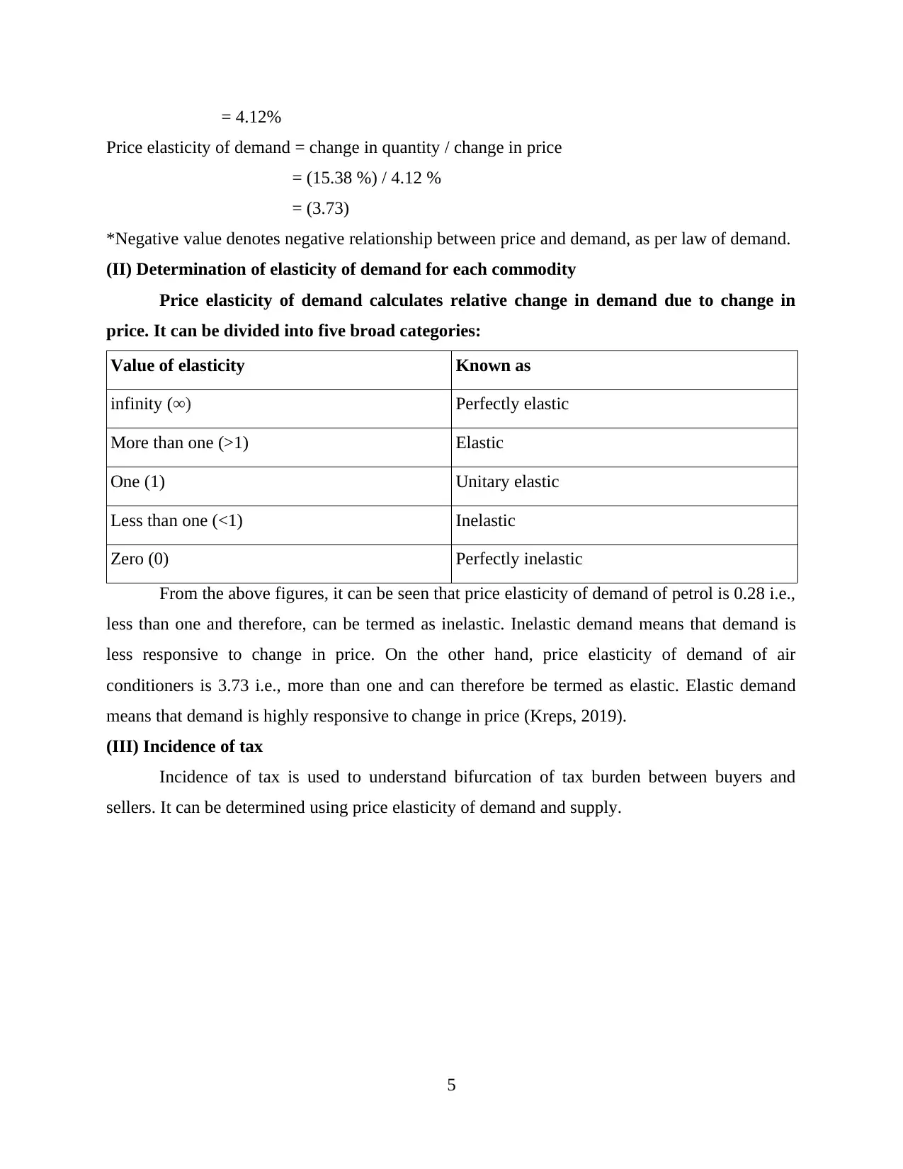
From the above figures, it can be seen that price elasticity of demand of petrol is 0.28 i.e.,
less than one and therefore, can be termed as inelastic. Inelastic demand means that demand is
less responsive to change in price. On the other hand, price elasticity of demand of air
conditioners is 3.73 i.e., more than one and can therefore be termed as elastic. Elastic demand
means that demand is highly responsive to change in price (Kreps, 2019).
(III) Incidence of tax
Incidence of tax is used to understand bifurcation of tax burden between buyers and
sellers. It can be determined using price elasticity of demand and supply.
5
Price elasticity of demand = change in quantity / change in price
= (15.38 %) / 4.12 %
= (3.73)
*Negative value denotes negative relationship between price and demand, as per law of demand.
(II) Determination of elasticity of demand for each commodity
Price elasticity of demand calculates relative change in demand due to change in
price. It can be divided into five broad categories:
Value of elasticity Known as
infinity (∞) Perfectly elastic
More than one (>1) Elastic
One (1) Unitary elastic
Less than one (<1) Inelastic
Zero (0) Perfectly inelastic
From the above figures, it can be seen that price elasticity of demand of petrol is 0.28 i.e.,
less than one and therefore, can be termed as inelastic. Inelastic demand means that demand is
less responsive to change in price. On the other hand, price elasticity of demand of air
conditioners is 3.73 i.e., more than one and can therefore be termed as elastic. Elastic demand
means that demand is highly responsive to change in price (Kreps, 2019).
(III) Incidence of tax
Incidence of tax is used to understand bifurcation of tax burden between buyers and
sellers. It can be determined using price elasticity of demand and supply.
5
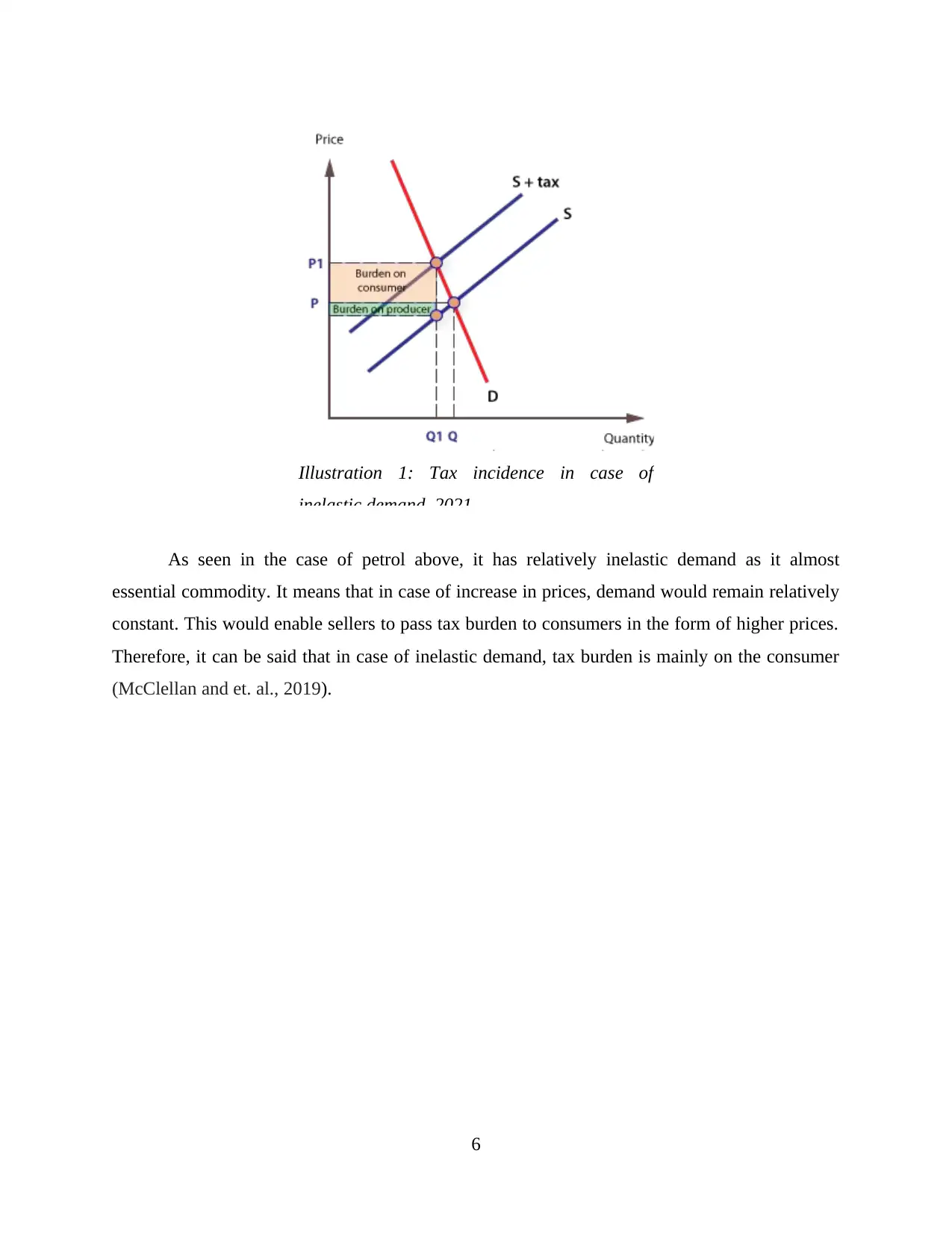
As seen in the case of petrol above, it has relatively inelastic demand as it almost
essential commodity. It means that in case of increase in prices, demand would remain relatively
constant. This would enable sellers to pass tax burden to consumers in the form of higher prices.
Therefore, it can be said that in case of inelastic demand, tax burden is mainly on the consumer
(McClellan and et. al., 2019).
6
Illustration 1: Tax incidence in case of
inelastic demand, 2021
⊘ This is a preview!⊘
Do you want full access?
Subscribe today to unlock all pages.
Trusted by 1+ million students worldwide
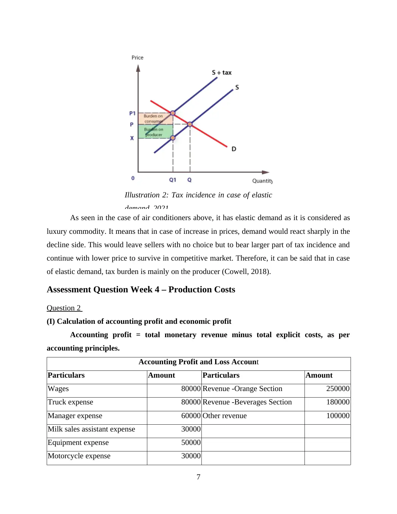
As seen in the case of air conditioners above, it has elastic demand as it is considered as
luxury commodity. It means that in case of increase in prices, demand would react sharply in the
decline side. This would leave sellers with no choice but to bear larger part of tax incidence and
continue with lower price to survive in competitive market. Therefore, it can be said that in case
of elastic demand, tax burden is mainly on the producer (Cowell, 2018).
Assessment Question Week 4 – Production Costs
Question 2
(I) Calculation of accounting profit and economic profit
Accounting profit = total monetary revenue minus total explicit costs, as per
accounting principles.
Accounting Profit and Loss Account
Particulars Amount Particulars Amount
Wages 80000 Revenue -Orange Section 250000
Truck expense 80000 Revenue -Beverages Section 180000
Manager expense 60000 Other revenue 100000
Milk sales assistant expense 30000
Equipment expense 50000
Motorcycle expense 30000
7
Illustration 2: Tax incidence in case of elastic
demand, 2021
Paraphrase This Document
Need a fresh take? Get an instant paraphrase of this document with our AI Paraphraser
Interest Expense (@8%) 3200
Net profit 196800
530000 530000
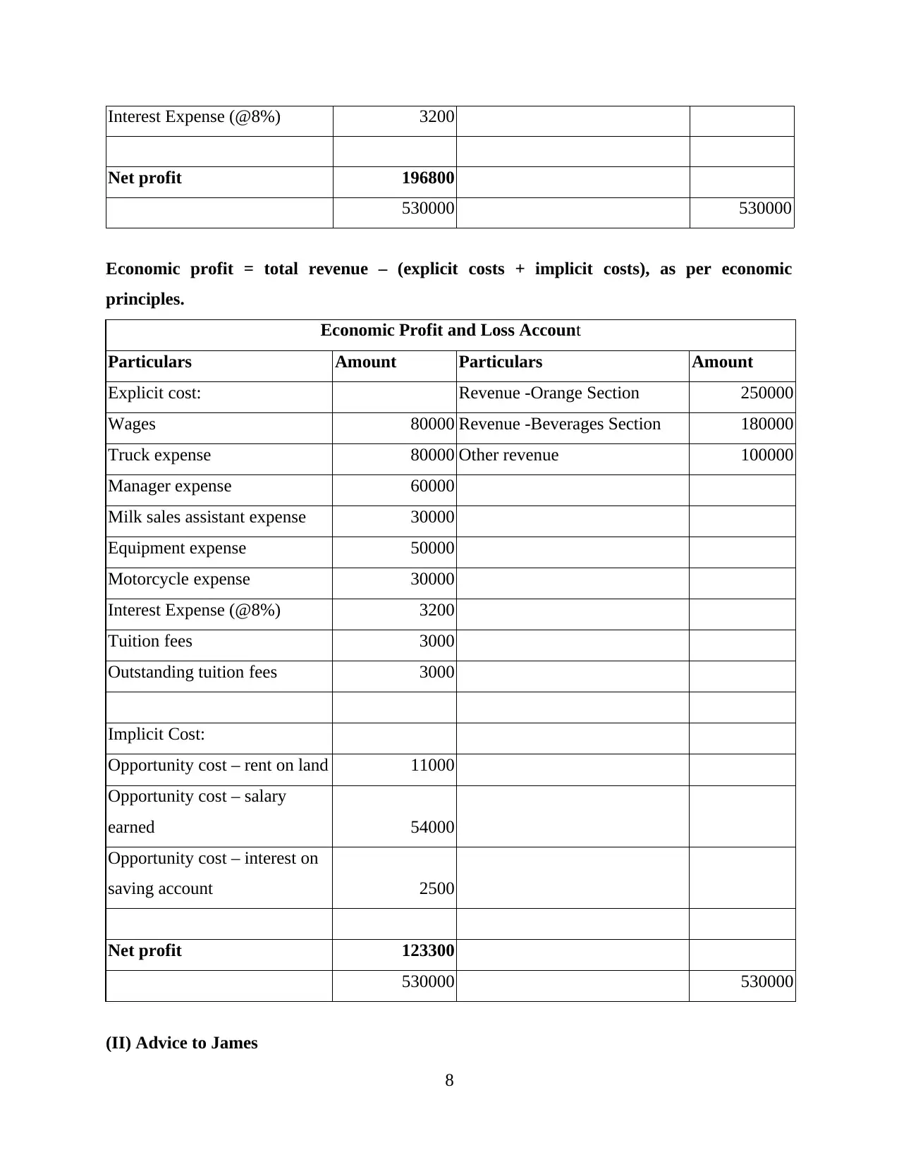
Economic profit = total revenue – (explicit costs + implicit costs), as per economic
principles.
Economic Profit and Loss Account
Particulars Amount Particulars Amount
Explicit cost: Revenue -Orange Section 250000
Wages 80000 Revenue -Beverages Section 180000
Truck expense 80000 Other revenue 100000
Manager expense 60000
Milk sales assistant expense 30000
Equipment expense 50000
Motorcycle expense 30000
Interest Expense (@8%) 3200
Tuition fees 3000
Outstanding tuition fees 3000
Implicit Cost:
Opportunity cost – rent on land 11000
Opportunity cost – salary
earned 54000
Opportunity cost – interest on
saving account 2500
Net profit 123300
530000 530000
(II) Advice to James
8
Net profit 196800
530000 530000
Economic profit = total revenue – (explicit costs + implicit costs), as per economic
principles.
Economic Profit and Loss Account
Particulars Amount Particulars Amount
Explicit cost: Revenue -Orange Section 250000
Wages 80000 Revenue -Beverages Section 180000
Truck expense 80000 Other revenue 100000
Manager expense 60000
Milk sales assistant expense 30000
Equipment expense 50000
Motorcycle expense 30000
Interest Expense (@8%) 3200
Tuition fees 3000
Outstanding tuition fees 3000
Implicit Cost:
Opportunity cost – rent on land 11000
Opportunity cost – salary
earned 54000
Opportunity cost – interest on
saving account 2500
Net profit 123300
530000 530000
(II) Advice to James
8
Accounting profit only takes into account explicit monetary costs and incomes while
economic profit is the profit that encompasses not only explicit costs but also implicit costs and
incomes and is therefore, generally lesser than accounting profit. It accounts for a complete
picture and hence, it is a better parameter to check profitability and financial viability of the firm
(McConnell, Brue and Flynn, 2018). Economic profit can be positive, negative or zero and if
only, the economic profit is positive, should the firm continue. In the provided case, firm of
James has an economic profit of $123,300 which shows that his kiosk business is a profitable
venture. Also, the profit earned is higher than his annual salary. Therefore, it is suggested that
James should continue with kiosk business.
Assessment Question Week 5 and 6 – Market Structure
Question 3
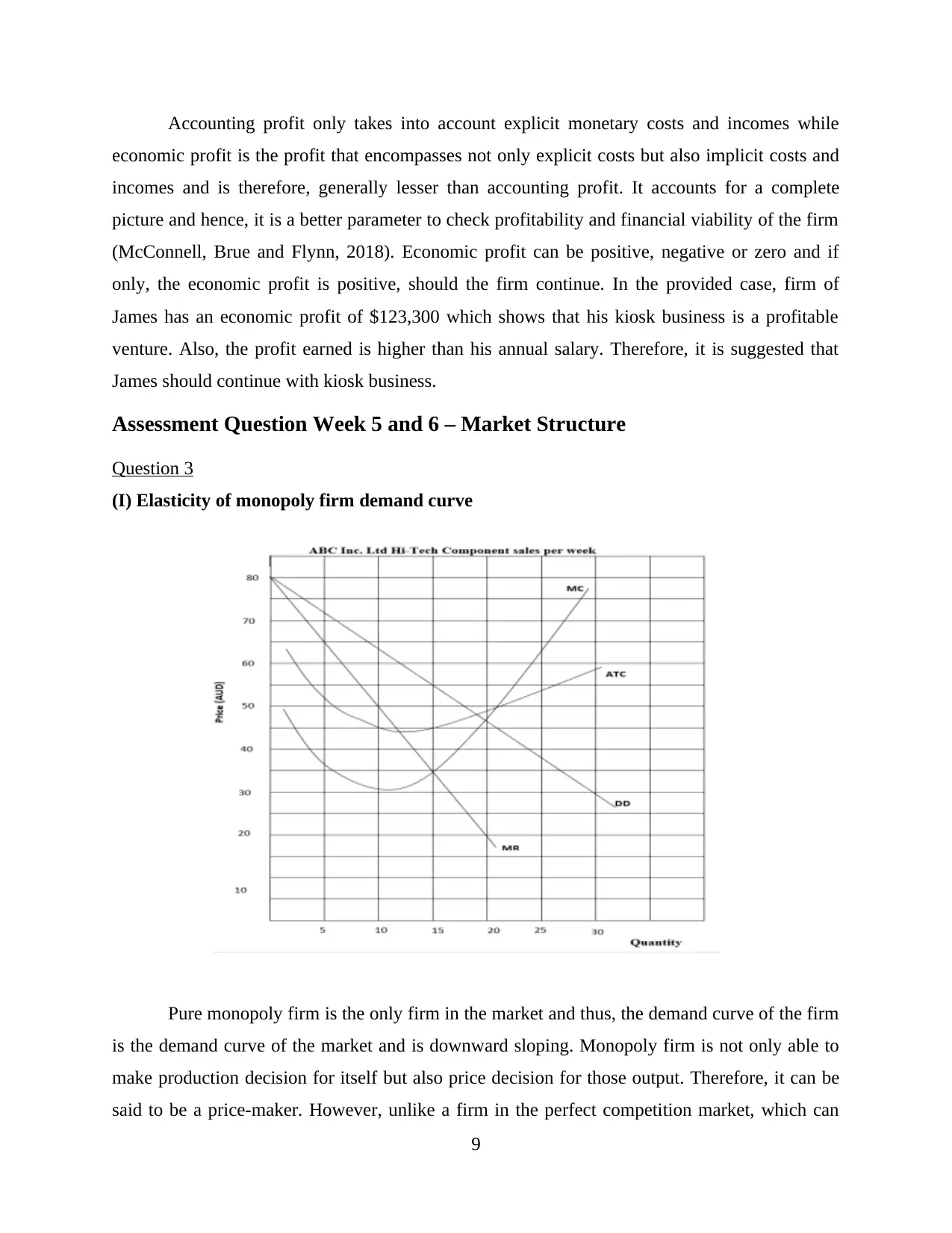
(I) Elasticity of monopoly firm demand curve
Pure monopoly firm is the only firm in the market and thus, the demand curve of the firm
is the demand curve of the market and is downward sloping. Monopoly firm is not only able to
make production decision for itself but also price decision for those output. Therefore, it can be
said to be a price-maker. However, unlike a firm in the perfect competition market, which can
9
economic profit is the profit that encompasses not only explicit costs but also implicit costs and
incomes and is therefore, generally lesser than accounting profit. It accounts for a complete
picture and hence, it is a better parameter to check profitability and financial viability of the firm
(McConnell, Brue and Flynn, 2018). Economic profit can be positive, negative or zero and if
only, the economic profit is positive, should the firm continue. In the provided case, firm of
James has an economic profit of $123,300 which shows that his kiosk business is a profitable
venture. Also, the profit earned is higher than his annual salary. Therefore, it is suggested that
James should continue with kiosk business.
Assessment Question Week 5 and 6 – Market Structure
Question 3
(I) Elasticity of monopoly firm demand curve
Pure monopoly firm is the only firm in the market and thus, the demand curve of the firm
is the demand curve of the market and is downward sloping. Monopoly firm is not only able to
make production decision for itself but also price decision for those output. Therefore, it can be
said to be a price-maker. However, unlike a firm in the perfect competition market, which can
9
⊘ This is a preview!⊘
Do you want full access?
Subscribe today to unlock all pages.
Trusted by 1+ million students worldwide
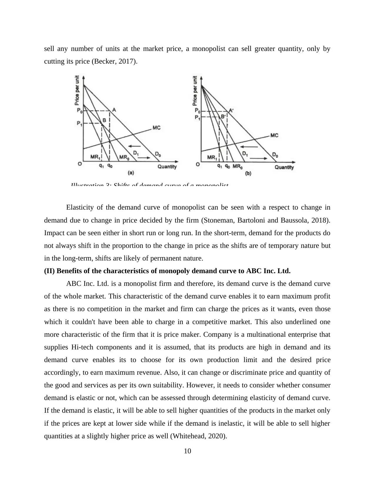
sell any number of units at the market price, a monopolist can sell greater quantity, only by
cutting its price (Becker, 2017).
Elasticity of the demand curve of monopolist can be seen with a respect to change in
demand due to change in price decided by the firm (Stoneman, Bartoloni and Baussola, 2018).
Impact can be seen either in short run or long run. In the short-term, demand for the products do
not always shift in the proportion to the change in price as the shifts are of temporary nature but
in the long-term, shifts are likely of permanent nature.
(II) Benefits of the characteristics of monopoly demand curve to ABC Inc. Ltd.
ABC Inc. Ltd. is a monopolist firm and therefore, its demand curve is the demand curve
of the whole market. This characteristic of the demand curve enables it to earn maximum profit
as there is no competition in the market and firm can charge the prices as it wants, even those
which it couldn't have been able to charge in a competitive market. This also underlined one
more characteristic of the firm that it is price maker. Company is a multinational enterprise that
supplies Hi-tech components and it is assumed, that its products are high in demand and its
demand curve enables its to choose for its own production limit and the desired price
accordingly, to earn maximum revenue. Also, it can change or discriminate price and quantity of
the good and services as per its own suitability. However, it needs to consider whether consumer
demand is elastic or not, which can be assessed through determining elasticity of demand curve.
If the demand is elastic, it will be able to sell higher quantities of the products in the market only
if the prices are kept at lower side while if the demand is inelastic, it will be able to sell higher
quantities at a slightly higher price as well (Whitehead, 2020).
10
Illustration 3: Shifts of demand curve of a monopolist
Paraphrase This Document
Need a fresh take? Get an instant paraphrase of this document with our AI Paraphraser
(III) Profit in the long run
It is assumed that cost curve and demand curve of the company results in the economic
profit for the firm in short-term. In the long-term, it is assumed that all other factors are constant
and this means that company is still only firm and enjoys monopoly in the market. Monopolist
still have economies of scale which empowers them to have lower long-run average cost and
good demand, when combined with it, will enable the ABC Inc. Ltd. to earn profits in the long
term. However, in the long run, if the condition of ceteris peribus does not work, it is highly
possible that new firms will enter the market and, in that case, it is possible that long-term profit
f the company reduces or either reduced to zero.
(IV) Effects of ABC Inc. Ltd. On consumers
ABC Inc. Ltd. is a monopoly and like other monopolists restricts the option for its
consumers to choose out of multiple options and since there is no alternative option for the
customer to buy the commodity if it is needed, it will have to purchase the product even on
higher prices than expected. Moreover, company can restrict its output in the market according
to its own suitability and this would leave the consumers with no option than waiting for the
product, even at the cost of harming its own efficiency and effectiveness of operations. All these
benefits at the end of the company not only restricts the choices of the consumers but also
reduces their sovereignty. In addition, it reduces consumer surplus. Consumer surplus is derived
whenever the price a consumer actually pays is less than they are prepared to pay (Kirschen and
Strbac, 2018). Reduced consumer surplus affects the demand of the firm in long run as now the
consumer would only demand as much as they require and if the ABC Inc. Ltd. wants to increase
its sales, it has to compulsorily reduce the price to attract them.
Assessment Question Week 7 and 8 – Measuring the size of the economy
Question 4
(I) Calculation of nominal GDP and real GDP in 2016
Gross Domestic Product (GDP) of an economy is the total market value or monetary
value of all the finished goods and services that have been produced within the economy in a
definite time period (Welch and Welch, 2016). GDP is calculated and reported by Australian
Bureau of Statistics (ABS) at a quarterly interval. It collects data from government agencies,
11
companies and household to calculate GDP in three different ways – production (P), income (I)
and expenditure (E), which are mentioned below:
GDP(P) – It includes sum total value from all goods and services produced.
GDP (I) – It includes total income that has been generated by employees and businesses
(net of taxes minus subsidies)
GDP (E) – It includes total value of spending by businesses, consumers and government
on final goods and services.
These three different ways estimate almost same things but in Australia, ABS uses average
of three to arrive at GDP (A).
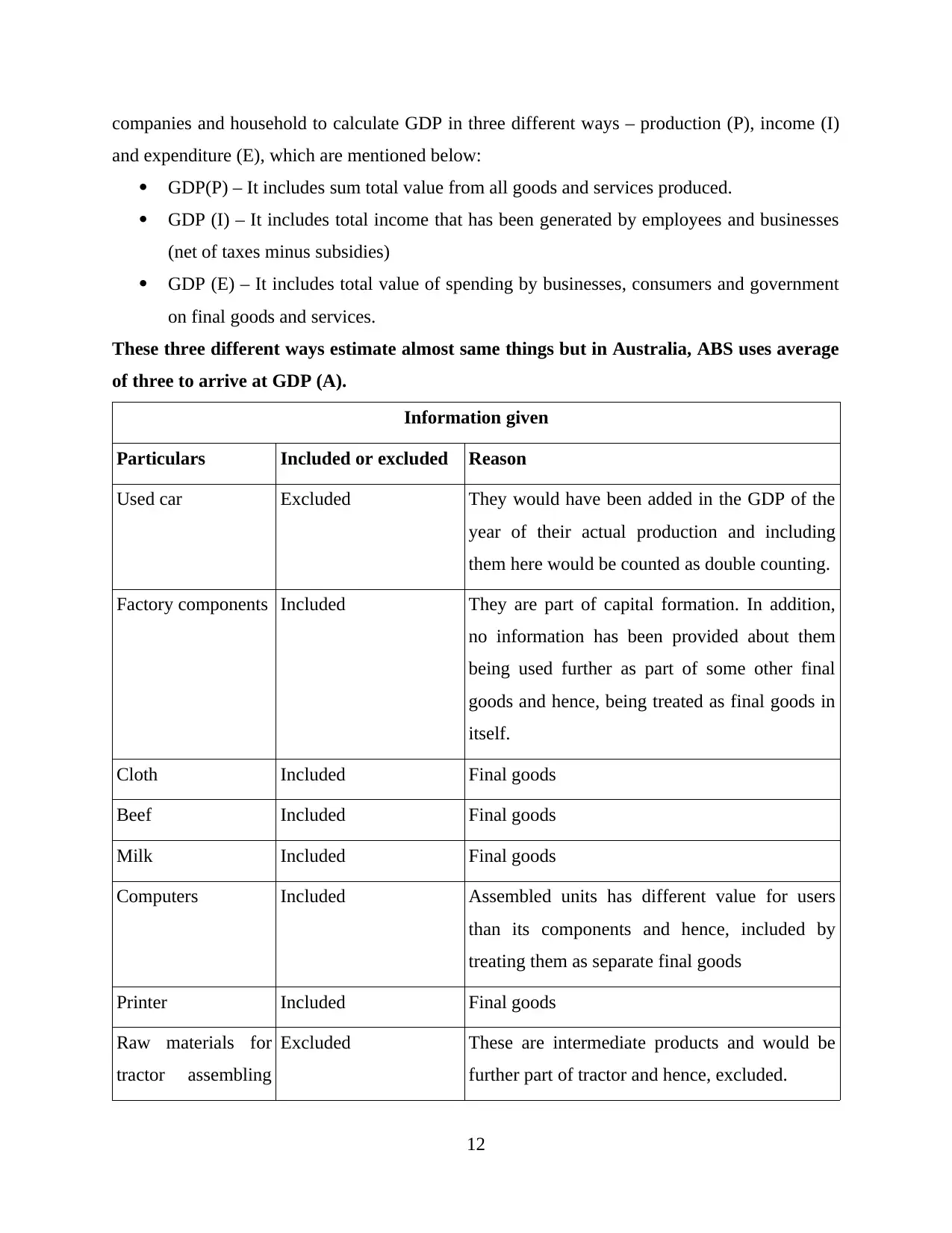
Information given
Particulars Included or excluded Reason
Used car Excluded They would have been added in the GDP of the
year of their actual production and including
them here would be counted as double counting.
Factory components Included They are part of capital formation. In addition,
no information has been provided about them
being used further as part of some other final
goods and hence, being treated as final goods in
itself.
Cloth Included Final goods
Beef Included Final goods
Milk Included Final goods
Computers Included Assembled units has different value for users
than its components and hence, included by
treating them as separate final goods
Printer Included Final goods
Raw materials for
tractor assembling
Excluded These are intermediate products and would be
further part of tractor and hence, excluded.
12
and expenditure (E), which are mentioned below:
GDP(P) – It includes sum total value from all goods and services produced.
GDP (I) – It includes total income that has been generated by employees and businesses
(net of taxes minus subsidies)
GDP (E) – It includes total value of spending by businesses, consumers and government
on final goods and services.
These three different ways estimate almost same things but in Australia, ABS uses average
of three to arrive at GDP (A).
Information given
Particulars Included or excluded Reason
Used car Excluded They would have been added in the GDP of the
year of their actual production and including
them here would be counted as double counting.
Factory components Included They are part of capital formation. In addition,
no information has been provided about them
being used further as part of some other final
goods and hence, being treated as final goods in
itself.
Cloth Included Final goods
Beef Included Final goods
Milk Included Final goods
Computers Included Assembled units has different value for users
than its components and hence, included by
treating them as separate final goods
Printer Included Final goods
Raw materials for
tractor assembling
Excluded These are intermediate products and would be
further part of tractor and hence, excluded.
12
⊘ This is a preview!⊘
Do you want full access?
Subscribe today to unlock all pages.
Trusted by 1+ million students worldwide
1 out of 23
Related Documents


Your All-in-One AI-Powered Toolkit for Academic Success.
+13062052269
info@desklib.com
Available 24*7 on WhatsApp / Email
![[object Object]](/_next/static/media/star-bottom.7253800d.svg)
Unlock your academic potential
Copyright © 2020–2026 A2Z Services. All Rights Reserved. Developed and managed by ZUCOL.