Economics Assignment: Analyzing Costs, Pricing, and Strategies
VerifiedAdded on 2020/05/28
|8
|2492
|179
Homework Assignment
AI Summary
This economics assignment provides detailed solutions to several problems. The first problem analyzes the impact of an extra shift on marginal costs and subsequent pricing decisions, differentiating between variable and fixed costs. The second solution examines the benefits of a diversified supplier base and product offerings for a business. The third solution explores the implications of a business not making profits on weekends, considering both variable and fixed costs and potential courses of action. The fourth solution discusses price discrimination strategies, using the example of an amusement park. The fifth solution applies game theory to a scenario involving a firm and its supplier, determining the Nash equilibrium. The sixth solution addresses decision-making under demand uncertainty, calculating probabilities for different outcomes. Finally, the seventh solution analyzes expected winnings based on bid values and probabilities.
NAME
USQ STUDENT NUMBER
Page 1 of 8
USQ STUDENT NUMBER
Page 1 of 8
Paraphrase This Document
Need a fresh take? Get an instant paraphrase of this document with our AI Paraphraser
ANSWER 1: We note that the question is asking for two answers. One is the effect of an
extra shift on short run marginal costs. The second is the consequent effect on pricing
decisions due to this change in marginal costs. The key lies in differentiating between
variable and fixed costs. Variable costs of production are costs that vary with output level.
Typically wages are a good example as we need more workers who are paid in the form of
wages to produce more. Fixed costs are costs that do not vary with how much is produced.
A good example is rent paid for the factory premises. In this case of our firm a new shift will
imply more workers and attendant usage of raw materials and electricity ( to possibly run
the machines). The added costs of wages of the workers in this shift and the costs of
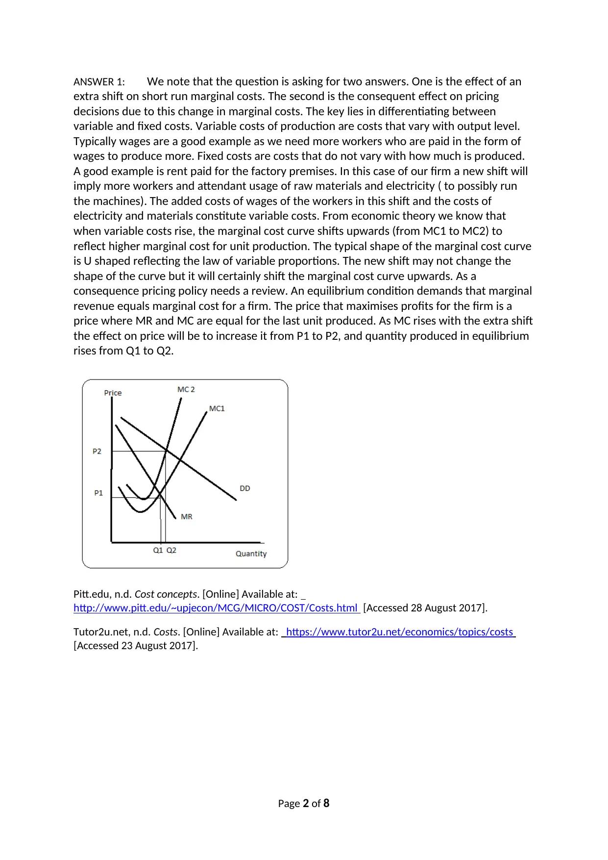
electricity and materials constitute variable costs. From economic theory we know that
when variable costs rise, the marginal cost curve shifts upwards (from MC1 to MC2) to
reflect higher marginal cost for unit production. The typical shape of the marginal cost curve
is U shaped reflecting the law of variable proportions. The new shift may not change the
shape of the curve but it will certainly shift the marginal cost curve upwards. As a
consequence pricing policy needs a review. An equilibrium condition demands that marginal
revenue equals marginal cost for a firm. The price that maximises profits for the firm is a
price where MR and MC are equal for the last unit produced. As MC rises with the extra shift
the effect on price will be to increase it from P1 to P2, and quantity produced in equilibrium
rises from Q1 to Q2.
Pitt.edu, n.d. Cost concepts. [Online] Available at:
http://www.pitt.edu/~upjecon/MCG/MICRO/COST/Costs.html [Accessed 28 August 2017].
Tutor2u.net, n.d. Costs. [Online] Available at: https://www.tutor2u.net/economics/topics/costs
[Accessed 23 August 2017].
Page 2 of 8
extra shift on short run marginal costs. The second is the consequent effect on pricing
decisions due to this change in marginal costs. The key lies in differentiating between
variable and fixed costs. Variable costs of production are costs that vary with output level.
Typically wages are a good example as we need more workers who are paid in the form of
wages to produce more. Fixed costs are costs that do not vary with how much is produced.
A good example is rent paid for the factory premises. In this case of our firm a new shift will
imply more workers and attendant usage of raw materials and electricity ( to possibly run
the machines). The added costs of wages of the workers in this shift and the costs of
electricity and materials constitute variable costs. From economic theory we know that
when variable costs rise, the marginal cost curve shifts upwards (from MC1 to MC2) to
reflect higher marginal cost for unit production. The typical shape of the marginal cost curve
is U shaped reflecting the law of variable proportions. The new shift may not change the
shape of the curve but it will certainly shift the marginal cost curve upwards. As a
consequence pricing policy needs a review. An equilibrium condition demands that marginal
revenue equals marginal cost for a firm. The price that maximises profits for the firm is a
price where MR and MC are equal for the last unit produced. As MC rises with the extra shift
the effect on price will be to increase it from P1 to P2, and quantity produced in equilibrium
rises from Q1 to Q2.
Pitt.edu, n.d. Cost concepts. [Online] Available at:
http://www.pitt.edu/~upjecon/MCG/MICRO/COST/Costs.html [Accessed 28 August 2017].
Tutor2u.net, n.d. Costs. [Online] Available at: https://www.tutor2u.net/economics/topics/costs
[Accessed 23 August 2017].
Page 2 of 8
Answer 2:
We need to analyse the shift from 1 supplier to multiple suppliers for Nora Nicest Knick
Knacks. There is another change that has occurred along with this supplier change- Nora has
expanded her product offering to go beyond tee-shirts, and it now includes cups, mugs, key
chains and many other items. This expansion in offerings is beneficial as Nora is able to cater
to a wider customer group. This in itself will allow her to create more value as she caters to
more customers with wider choices. She will be able to capture a larger part of this value
creation with the right kind of pricing, keeping in mind consumer preferences.
She can also gain value created from the expansion in supplier base. She is no longer
dependent on a single supplier who could get away by capturing larger share of the value
created due to the supplier-buyer relation. Multiple suppliers allows her to be flexible in her
choice of suppliers and consequently she can take away a larger part of the value created
from each supplier as compared to the value she got from a single supplier.
Tescari, F.C. & Brito, A.L.L., 2016. VALUE CREATION AND CAPTURE IN Buyer Seller Relationships.
[Online] Available at: http://www.scielo.br/pdf/rae/v56n5/0034-7590-rae-56-05-0474.pdf
[Accessed 8 Jan 2018].
Page 3 of 8
⊘ This is a preview!⊘
Do you want full access?
Subscribe today to unlock all pages.
Trusted by 1+ million students worldwide
Answer 3: The question tells us that Hank Honkytonks(HH) is not making profits on
weekends, after charging a $5 charge from each patron. This charge is the revenue for HH.
Its profits can be understood when we look at its costs as well, since profits are the
difference between revenues and costs. Since we have no information on costs but know of
its losses it is clear that costs exceed revenues. In this scenario the future course of action
depends on variable and fixed costs components of costs. We distinguish between 2 cases.
Case1: Revenues cover only the variable costs of running HH on weekends. This implies that
variable Costs are covered by the revenues generated from $5 entry fee. The losses are
therefore equal or less than the fixed costs. HH can continue its weekends programs in the
hope that in the long run more patrons will come in and revenues will be enough to cover
fixed costs as well. It can also seek to lower its fixed costs; a possibility is to take on a
different band that charges lesser from HH. Alternatively HH can negotiate with the band to
charge lower amount or charge in line with the number of patrons. The last option will
convert the band charges to variable costs, wiping out losses.
Case 2: If the revenues are not covering the variable costs then HH has no option but to
close down/ shut down operations. This conclusion is based on economic theory which
relies on differentiating between fixed and variable costs. It also assumes that the firm can
make no changes to its costs or revenues.
If we allow some changes then things can be different. For example HH can try to increase
revenues and/or lower costs. One way to increase revenues is to increase entry fee without
loss of patrons. If the demand for HH is inelastic then a rise in fees will not lower the
number of patrons, and will boost revenues as well. It can also lower costs by changing the
band that plays on weekends or renegotiating with the band to charge a lower price. It may
also work on partnership basis with the band where revenues/losses are shared, so that
fixed costs can be lowered.
Guitierrez, P.H. & Dalsted, N.L., n.d. Break even method. [Online] Available at:
http://extension.colostate.edu/topic-areas/agriculture/break-even-method-of-investment-analysis-
3-759-2/ [Accessed 2 Jan 2018].
Mankiw, N.G., n.d. Principles of Economics. In markets and welfare. 6th ed. Cengagebrain.com.
pp.160-62.
Page 4 of 8
Paraphrase This Document
Need a fresh take? Get an instant paraphrase of this document with our AI Paraphraser
Answer 4: the answer here lies in the concept of price discrimination. It refers to a
concept where a firm charges a different price from each consumer depending on a variety
of aspects of the consumer – his preferences, time of use, quantity bought and willingness
to buy. The Six Flags Over Texas amusement park would like to charge a higher price from
the tourists who visit it, and a lower price from the local people. This is possible as tourists
have a higher willingness to pay for the park attractions, as compared to local people who
have little novelty value for these attractions, and are willing to pay a lower price for the
park attractions. The discount is meant for locals who may visit the park as their willingness
to pay is lower. The use of the Coke can effectively lowers the price of entry into the park for
such locals whose willingness to pay is lower than tourists. Such locals may not visit the park
at full price as the price exceeds their willingness to pay for the park attractions.
The tie up with Coke is purely to attract more customers as Coke sells widely. A discount of
$5 may encourage Coke drinking locals and tourists to visit the park. However it is also
desirable that this $5 discount is not used by tourists, as they are willing to pay more. So the
limit of 20 mile radius is imposed to limit the use of this scheme by tourists from far away.
This implies that the park considers people in this radius to be locals who may be
encouraged to use the Coke can to get cheaper entry. Tourists can also use the discount, but
they will have to be in the 20 mile radius to be able to buy the can.
Aggarwal, P., n.d. Price elasticity of demand. [Online] Available
athttps://www.intelligenteconomist.com/price-elasticity-of-demand/ [Accessed 6 Jan 2018].
Economicsonline.co.uk, n.d. Price discrimination. [Online] Available
athttp://www.economicsonline.co.uk/Business_economics/Price_discrimination.html [Accessed 2
Jan 2018].
Page 5 of 8
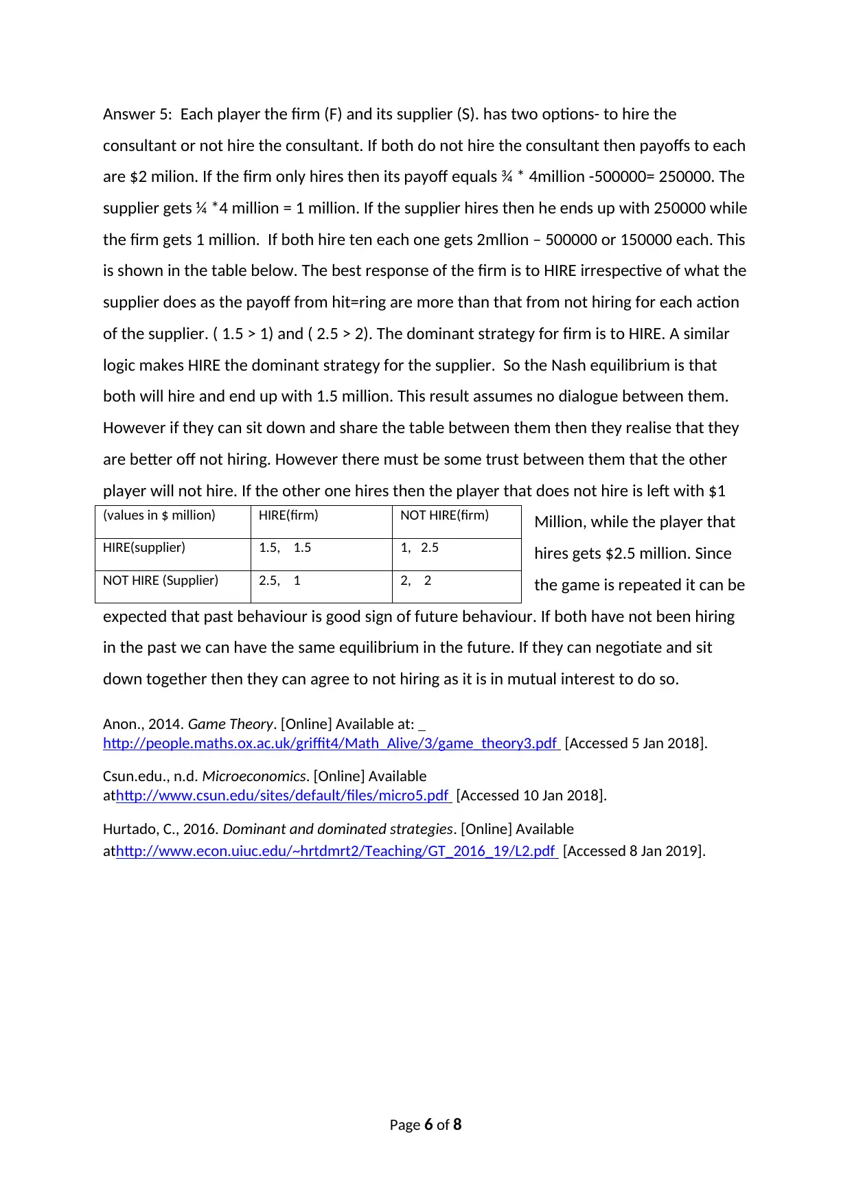
Answer 5: Each player the firm (F) and its supplier (S). has two options- to hire the
consultant or not hire the consultant. If both do not hire the consultant then payoffs to each
are $2 milion. If the firm only hires then its payoff equals ¾ * 4million -500000= 250000. The
supplier gets ¼ *4 million = 1 million. If the supplier hires then he ends up with 250000 while
the firm gets 1 million. If both hire ten each one gets 2mllion – 500000 or 150000 each. This
is shown in the table below. The best response of the firm is to HIRE irrespective of what the
supplier does as the payoff from hit=ring are more than that from not hiring for each action
of the supplier. ( 1.5 > 1) and ( 2.5 > 2). The dominant strategy for firm is to HIRE. A similar
logic makes HIRE the dominant strategy for the supplier. So the Nash equilibrium is that
both will hire and end up with 1.5 million. This result assumes no dialogue between them.
However if they can sit down and share the table between them then they realise that they
are better off not hiring. However there must be some trust between them that the other
player will not hire. If the other one hires then the player that does not hire is left with $1
Million, while the player that
hires gets $2.5 million. Since
the game is repeated it can be
expected that past behaviour is good sign of future behaviour. If both have not been hiring
in the past we can have the same equilibrium in the future. If they can negotiate and sit
down together then they can agree to not hiring as it is in mutual interest to do so.
Anon., 2014. Game Theory. [Online] Available at:
http://people.maths.ox.ac.uk/griffit4/Math_Alive/3/game_theory3.pdf [Accessed 5 Jan 2018].
Csun.edu., n.d. Microeconomics. [Online] Available
athttp://www.csun.edu/sites/default/files/micro5.pdf [Accessed 10 Jan 2018].
Hurtado, C., 2016. Dominant and dominated strategies. [Online] Available
athttp://www.econ.uiuc.edu/~hrtdmrt2/Teaching/GT_2016_19/L2.pdf [Accessed 8 Jan 2019].
Page 6 of 8
(values in $ million) HIRE(firm) NOT HIRE(firm)
HIRE(supplier) 1.5, 1.5 1, 2.5
NOT HIRE (Supplier) 2.5, 1 2, 2
⊘ This is a preview!⊘
Do you want full access?
Subscribe today to unlock all pages.
Trusted by 1+ million students worldwide
Answer 6:
Demand is uncertain and this forces two options on the buyer here. One is to have a poor
design choice and the other is to choose a design in high demand. If a poorly demanded
design is ordered then the losses equal $200000. The other option fetches a profit of
$300000. These values are the payoffs from two alternate choices in an atmosphere of
uncertainty.
Next we need to have an objective in mind in terms of expected profits. For example the
buyer may want to try to avoid any losses, so that expected profits can be equated to zero.
Let p stand for the probability of choosing poorly demanded design, while 1-p is the chance
for a high demand design to be ordered.
Expected profits is the sum of weighted profits( or losses) where the weights are the
probabilities associated with each choice.
So expected profits = p*300000 +(1-p)*(-200000) = 0
A minus sign signifies loss of 200000
Solving this we get p = 2/5 or 40%.
So the probability of a design’s success must be 40% for the firm to order it. This figure
assumes that the firm is aiming at zero loss / zero profit.
If the objective is changed to ( say) an expected profit of 50000 then we have
expected profits = p*300000 +(1-p)*(-200000) = 50000
now p= 0.5 or 50%.
Anon., n.d. Decesion Theory. [Online] Available at:
https://people.richland.edu/james/summer02/m160/decision.html [Accessed 7 Jan 2018].
Page 7 of 8
Paraphrase This Document
Need a fresh take? Get an instant paraphrase of this document with our AI Paraphraser
Answer 7:
The expected winnings from an event depend on two things. The first is the amount of
winnings promised if the participant wins and the associated loss if she does not win. The
second requirement is the probability or chances of winning itself, along with the list of all
possible options (win, loss or nothing). In this case we are not exactly winning or losing, but
the analysis is similar. There are two options here- high value bid ( $70) and low value
bid( $50). The chances of a high value bid are 0.5 as we have 2 bidders out of 4 who have a
value of $70. The winnings/losses from the bid are the value of the bid made- $70 or $50.
The expected winning bid equals the weighted average of all possible bids, where the
weights are the probability of the bids.
Expected winning bid= Sum of product of the bid amount and the probability/chance of this
amount
= .5*70 +.5*50 = $60.
The number of bidders does not directly form part of the answer as we have used it to
calculate the chances of each possible bid value. Assume that 3 bidders had a value of $70
and one bidder has $50 value. Then the probability of $70 bid would be ¾=0.75 so that
expected winning bid would equal .75*70 +.25*50 = 52.5 + 12.5 = $65
Mausam, n.d. Fundamentals of Decesion theory. [Online] Available at:
https://courses.cs.washington.edu/courses/cse573/12au/slides/05a-decisiontheory.pdf [Accessed 9
Jan 2018].
siue.edu, n.d. A very fast intro to decesion theory. [Online] Available
athttp://www.siue.edu/~evailat/decision.htm [Accessed 8 Jan 2018].
Page 8 of 8
1 out of 8
Related Documents


Your All-in-One AI-Powered Toolkit for Academic Success.
+13062052269
info@desklib.com
Available 24*7 on WhatsApp / Email
![[object Object]](/_next/static/media/star-bottom.7253800d.svg)
Unlock your academic potential
Copyright © 2020–2026 A2Z Services. All Rights Reserved. Developed and managed by ZUCOL.